


MOLCAS manual: Next: 8.48 surfacehop Up: 8. Programs Previous: 8.46 single_aniso
|
| File | Contents |
| RUNFILE | File for communication of auxiliary information. If a computed Hessian is available on this file it will be used rather than the approximate Hessian generated by Slapaf. |
| RUNFILE2 | File for communication of auxiliary information of the "ground state" in case of minimum energy cross point optimizations. |
| RUNOLD | File for communication of auxiliary information for reading an old Hessian matrix from a previous geometry optimization. |
8.47.3.2 Output files
In addition to the standard output file SlapAf will use the following output files.
| File | Contents |
| RUNFILE | File for communication of auxiliary information. |
| RUNFILE2 | File for communication of auxiliary information of the "ground state" in case of minimum energy cross point optimizations. |
| MD_GEO | Molden input file for geometry optimization analysis. |
| MD_MEP | Molden input file for minimum energy path (MEP). |
| MD_SADDLE | Molden input file for energy path (MEP) of a Saddle TS optimization. |
| MD_IRC | Molden input file for intrinsic reaction coordinate analysis of a TS. |
| MD_FREQ | Molden input file for harmonic frequency analysis. |
| UNSYM | ASCII file where all essential information, like geometry, Hessian normal modes and dipole derivatives are stored. |
| STRUCTURE | Output file with a statistics of geometry optimization convergence. |
8.47.4 Input
SlapAf will as standard
provided with an energy and a corresponding gradient
update the geometry (optimize).
Possible update methods include different quasi-Newton methods.
The program will also provide for updates of the Hessian.
The program has a number of different variable metric methods available for
the Hessian update.
This section describes the input to the SlapAf program.
This section describes the input to the
SLAPAF program in the MOLCAS program system. The input starts
with the program name
&SLAPAF
There are no compulsory keywords
Optional convergence control keywords
| Keyword | Meaning |
| ITERations | Maximum number of iterations which will be allowed in the relaxation procedure. Default is 500 iterations, however, if environment variable MOLCAS_MAXITER has been exported by the user this is the assumed default value. |
| THRShld | Enter two real numbers which specifies the convergence criterion with respect to the energy change and the norm of the gradient. The defaults are 0.0 and 3.0D-4 au for Gaussian convergence criteria (which normally do not consider the energy change), and 1.0D-6 and 3.0D-4 for Baker criteria (see the BAKER keyword). |
| BAKEr | Activate convergence criteria according to Baker [162]. Default is to use the convergence criteria as in the Gaussian program [163]. |
| MAXStep | This keyword is followed by the value which defines the seed of largest change of the internal coordinates which will be accepted. A change which is larger is reduced to the max value. The value is dynamically modified each iterations. The default value is 0.3 au or rad. |
| CNWEight | Sets the maximum weight assigned to the fulfillment of the constraints, relative to the step taken in the complementary space for energy minimization. The step in the constraint space is truncated to be at most as large as the step in the minimization space, or half the maximum total step, whichever is larger, multiplied by this value. Default is 1.0. |
| TOLErance | Controls how strictly the constraints (if any) must be satisfied at convergence. The default value is very large, such that this criterion is always met, and only the gradient and maximum step (or energy difference) control convergence. If you set this keyword to some value, a constrained optimization will only converge if the maximum error in any constraint is lower than this number (in atomic units, and radians). |
Optional coordinate selection keywords
| Keyword | Meaning |
| CARTesian | Activate SlapAf to use the eigenvectors of the approximative Hessian expressed in Cartesian as the definition of the internal coordinates. The default is to use the FCW non-redundant internal coordinates. The Hessian will be modeled by the Hessian Model Functional. |
| INTErnal | This marks the start of the definition of the internal
coordinates. This section is always ended by the keyword
End of Internal.
For a complete description of this
keyword see the section
![[*]](crossref.png) .
This option will also use a diagonal matrix as default for
the Hessian matrix.
The default is to
use the FCW non-redundant internal coordinates. .
This option will also use a diagonal matrix as default for
the Hessian matrix.
The default is to
use the FCW non-redundant internal coordinates.
|
| HWRS | Use the force constant weighted (FCW) redundant space version of the nonredundant internal coordinates. This is the default. The Hessian will be modeled by the Hessian Model Functional. |
| NOHWrs | Disable the use of the force constant weighted redundant space version of the nonredundant internal coordinates. The default is to use the HWRS option. The Hessian will be modeled by the Hessian Model Functional. |
| FUZZ | When automatically generating the primitive internal coordinates, the system may end up in disconnected fragments, in which case additional bonds are defined between the fragments. This keyword controls how many inter-fragment bonds are added. Bonds are generated between the closest atoms of two fragments, and all pairs of atoms in separate fragments at a distance up to the specified value longer. The value can be followed with the unit BOHR or ANGSTROM. The default is 0.5 a.u. |
Optional Hessian update keywords
| Keyword | Meaning |
| HUPDate | Method used for updating the Hessian matrix. It must be one of:
|
| UORDer | Order the gradients and displacements vectors according to Schlegel prior to the update of the Hessian. Default is no reorder. |
| WINDow | Maximum number of previous iterations to include in the Hessian update. Default is 5. |
Optional optimization procedure keywords
| Keyword | Meaning |
| NOLIne | Disable line search. Default is to use line search for minima. |
| RATIonal | Activate geometry optimization using the restricted step Rational Functional optimization [166,167], this is the default. |
| C1-Diis | Activate geometry optimization using the C1-GDIIS method [168,169,170]. The default is to use the Rational Functional approach. |
| C2-Diis | Activate geometry optimization using the C2-GDIIS method [98]. The default is to use the Rational Functional approach. |
| DXDX | This option is associated to the use of the C1- and C2-GDIIS
procedures. This option will activate the computation of the
so-called error matrix elements as
 ,
where ,
where  is the displacement vector. is the displacement vector.
|
| DXG | This option is associated to the use of the C1- and C2-GDIIS
procedures. This option will activate the computation of the
so-called error matrix elements as
 ,
where is the displacement vector and g is the
gradient vector. ,
where is the displacement vector and g is the
gradient vector.
|
| GDX | See above. |
| GG | This option is associated to the use of the C1- and C2-GDIIS
procedures. This option will activate the computation of the
so-called error matrix elements as
 ,
where g is the gradient vector. This is the default. ,
where g is the gradient vector. This is the default.
|
| NEWTon | Activate geometry optimization using the standard quasi-Newton approach. The default is to use the Rational Functional approach. |
| RS-P-rfo | Activate RS-P-RFO [167] as default for TS-search. Default is RS-I-RFO. |
| TS | Keyword for optimization of transition states. This flag will activate the use of the mode following rational functional approach [171]. The mode to follow can either be the one with the lowest eigenvalue (if positive it will be changed to a negative value) or by the eigenvector which index is specified by the MODE keyword (see below). The keyword will also activate the Murtagh-Sargent-Powell update of the Hessian and inactivate line search. This keyword will also enforce that the Hessian has the right index (i.e. one negative eigenvalue). |
| MODE | Specification of the Hessian eigenvector index, this mode will be followed by the mode following RF method for optimization of transition states. The keyword card is followed by a single card specifying the eigenvector index. |
| FINDTS | Enable a constrained optimization to release the constraints and locate a transition state if negative curvature is encountered and the gradient norm is below a specific threshold (see the GNRM option). Keyword TSCOnstraints should be used in combination with FINDTS. |
| TSCOnstraints | Specify constraints that will be active during the initial stage of an
optimization with FINDTS. When negative curvature and low
gradient are encountered, these constraints will be released and
other constraints will remain active. If this block is not given in
the input, all constraints will be released. The syntax of this
keyword is exactly like normal constraints, and it must be ended with
End of TSConstraints
(see section below).
|
| GNRM | Modify the gradient norm threshold associated with the FINDTS option. The actual threshold is specified on the subsequent line. The default value is 0.2. |
| MEP-search | Enable a minimum energy path (MEP) search. MEP is a valid synonym. |
| NMEP | Maximum number of points to find in a minimum energy path search or intrinsic reaction coordinate analysis. Synonym of NIRC. |
| MEPStep | The keyword is used to specify the step length done in the MEP search or IRC analysis. The step length can be followed with the unit BOHR or ANGSTROM. The default is 0.1 a.u. (in normalized mass-weighted coordinates). Synonym of IRCStep. |
| MEPType | Specifies what kind of constraint will be used for optimizing the points during the MEP search or IRC analysis. The possibilities are SPHERE, the default, which uses the Sphere constraint (each structure is at a given distance in coordinate space from the reference), or PLANE which uses the Transverse constraint (each structure is at a given distance from the hyperplane defined by the reference and the path direction). The reference structure changes at each step, according to the MEPAlgorithm keyword. Synonym of IRCType. |
| MEPAlgorithm | Selects the algorithm for a MEP search or IRC analysis. The possibilities are GS for the González-Schlegel algorithm, the default, or MB for the Müller-Brown algorithm. Synonym of IRCAlgorithm. |
| REFErence | The keyword is followed by a list of the symmetry unique coordinates (in au) of the origin of the hyper sphere. The default origin is the structure of the first iteration. |
| GRADient of reference | The keyword is followed by a list of the gradient vector components. This keyword is compulsory when using the Transverse kind of constraint. The optimization is performed in a space orthogonal to the given vector. |
| IRC | The keyword is used to perform an intrinsic reaction coordinate (IRC) analysis of a transition state structure. The analysis will follow the reaction path forward and backward until the energy increases. The keyword requires that the starting structure be that of a transition state and that the reaction vector be specified explicitly (check the keyword REACtion vector) or implicitly if it can be found on RUNOLD. Note that the user should not specify any explicit constraints! |
| NIRC | Maximum number of points to find in an intrinsic reaction coordinate analysis or minimum energy path search. Synonym of NMEP. |
| IRCStep | The keyword is used to specify the step length done in the IRC analysis or MEP search. The step length can be followed with the unit BOHR or ANGSTROM. The default is 0.1 a.u. (in normalized mass-weighted coordinates). Synonym of MEPStep. |
| IRCType | Specifies what kind of constraint will be used for optimizing the points during the IRC analysis or MEP search. The possibilities are SPHERE, the default, which uses the Sphere constraint (each structure is at a given distance in coordinate space from the reference), or PLANE which uses the Transverse constraint (each structure is at a given distance from the hyperplane defined by the reference and the path direction). The reference structure changes at each step, according to the IRCAlgorithm keyword. Synonym of MEPType |
| IRCAlgorithm | Selects the algorithm for a MEP search or IRC analysis. The possibilities are GS for the González-Schlegel algorithm, the default, or MB for the Müller-Brown algorithm. Synonym of MEPAlgorithm. |
| REACtion vector | The keyword is followed by the reaction vector specified as the Cartesian vector components on each of the symmetry unique atoms. |
Optional force constant keywords
| Keyword | Meaning |
| OLDForce | The Hessian matrix is read from the file RUNOLD. This Hessian is either an analytic or approximative Hessian updated by Slapaf. Note that for this option to work properly the type of internal coordinates must be the same! |
| FCONstant | Input of Hessian in internal coordinates.
There are two different syntaxes.
|
| XFCOnstant | Input of an external Hessian matrix in cartesian coordinates. The syntax is the same as for the FCONSTANT keyword. |
| NUMErical | This invokes as calculation of the force constant matrix by a two-point finite difference formula. The resulting force constant matrix is used for an analysis of the harmonic frequencies. Observe that in case of the use of internal coordinates defined as Cartesian coordinates that these has to be linear combinations which are free from translational and rotational components for the harmonic frequency analysis to be valid. Alternative: see keyword RowH in the section about Internal coordinates. |
| CUBIc | This invokes a calculation of the 2nd and the 3rd order force constant matrix by finite difference formula. |
| DELTa | This keyword is followed by a real number which defines the step length used in the finite differentiation. Default: 1.0D-2. |
| PRFC | The eigenvalues and eigenvectors of the Hessian matrix are printed. The internal coordinates definitions are also printed. |
| RHIDden | Define the hidden atoms selection radius in order to improve a QM/MM Hessian. It can be followed by Angstrom. |
Optional miscellaneous keywords
| Keyword | Meaning |
| CTOF | Coordinates TO Follow defines an internal coordinate whose values will be printed in the output during the optimization. Both the original and the new values will be printed. The keyword must be followed by the definition on the primitive coordinate. |
| RTRN | Maximum number of atoms for which bond lengths, angles and dihedral angles are listed, and the radius defining the maximum length of a bond follows. The latter is used as a threshold when printing out angles and dihedral angles. The length can be followed by Bohr or Angstrom which indicates the unit in which the length was specified, the default is Bohr. The default values are 15 and 3.0 au. |
| THERmochemistry | Request frequencies to be computed followed by an user specified thermochemical analysis. The keyword must be followed by different entries containing the Rotational Symmetry Number, the Pressure (in atm), and one entry per Temperature (in K) for which the thermochemistry will be calculated. The section is ended by the keyword End of PT. |
| DISOtope | Calculates frequencies modified for double isotopic substitution. |
| TRACk | Tries to follow electronic states during an optimization, by computing state overlaps with RASSI at each step. Root numbers selected with RlxRoot in RASSCF or with the ``EDiff'' constraint are only fixed in the first iteration, then the best-matching states are chosen. |
| LASTenergy | Specifies the quantum chemical method requested for the Last_Energy module (e.g., SCF, CASSCF, CASPT2, etc.) The keyword must be followed by the name of the module. Moreover, the EMIL command COPY needs to be used in the global input to provide a file named LASTEN, containing the input for the specified module. |
| NOLAst energy | Disables the call to the Last_Energy module when convergence is achieved.
|
Example: A complete set of input decks for a CASSCF geometry
optimization. These are the input decks for the optimization
of the enediyne molecule.
&GATEWAY
Title= Enediyne
Coord= $MOLCAS/Coord/enediyne.xyz
Basis= ANO-L-VQZP
Group= x z
> DoWhile
&SEWARD
&SCF
ITERATIONS= 30; Occupied= 9 8 2 1; Thresholds= 1.0d-8 1.0d-3 1.5d-3 0.2d-3; IVO
&RASSCF
Symmetry= 1; Spin= 1
NactEl= 12 0 0; Inactive= 7 7 0 0; Ras2= 3 3 3 3
Iterations= 50 50; CiRoot= 1 1; 1; Thrs= 1.0e-08 1.0e-05 1.0e-05
Lumorb
&SLAPAF; Iterations= 20
> EndDo
Example: Thermochemistry for an asymmetric top (Rotational Symmetry Number
= 1), at 1.0 atm and 273.15, 298.15, 398.15 and 498.15 K.
&SLAPAF; THERmochemistry= 1; 1.0; 273.15; 298.15; 398.15; 498.15; End of PT
End of input
8.47.4.1 Definition of internal coordinates or constraints
The input section defining the internal coordinates always start with the keyword Internal coordinates and the definition of the constraints starts with the keyword Constraints. Note that the latter is an input section for the GATEWAY module.
The input is always sectioned into two parts where the first section defines a set of primitive internal coordinates and the second part defines the actual internal coordinates as any arbitrary linear combination of the primitive internal coordinates that was defined in the first section. In case of constraints the second part does also assign values to the constraints.
In the first section we will refer to the atoms by their atom label (SEWARD will make sure that there is no redundancy). In case of symmetry one will have to augment the atom label with a symmetry operation in parenthesis in order to specify a symmetry related center. Note that the user only have to specify distinct internal coordinates (ALASKA will make the symmetry adaptation).
In the specification below rLabel is a user defined label with no more than 8 (eight) characters. The specifications atom1, atom2, atom3, and atom4 are the unique atom labels as specified in the input to SEWARD.
The primitive internal coordinates are defined as
- rLabel = Bond atom1 atom2 — a primitive internal coordinate rLabel is defined as the bond between center atom1 and atom2.
- rLabel = Angle atom1 atom2 atom3 — a primitive internal coordinate rLabel is defined as the angle between the bonds formed from connecting atom1 to atom2 and connecting atom2 to atom3.
- rLabel = LAngle(1) atom1 atom2 atom3 —
a primitive internal coordinate rLabel is defined as the linear angle
between the bonds formed from connecting atom1 to atom2 and
connecting atom2 to atom3. To define the direction of the angle the following
procedure is followed.
- – the three centers are linear,
- form a reference axis, R1, connecting atom1 and atom3,
- compute the number of zero elements, nR, in the reference vector,
- – nR=0,
a first perpendicular direction to the reference axis is formed by

followed by the projection
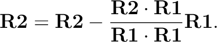
The second perpendicular direction completes the right-handed system. - – nR=1, a first perpendicular direction to the reference axis is defined by setting the element in R2 corresponding to the zero entry in R1 to unity. The second perpendicular direction completes the right-handed system.
- – nR=2, a first perpendicular direction to the reference axis is defined by setting the element corresponding to the first zero entry in R1 to unity. The second perpendicular direction completes the right-handed system.
- – nR=0,
a first perpendicular direction to the reference axis is formed by
- – the three centers are nonlinear, the first perpendicular direction is the one which is in the plane formed by atoms atom1, atom2, and atom3. The second perpendicular direction is taken as the direction perpendicular to the same plane.
- – the three centers are linear,
- rLabel = LAngle(2) atom1 atom2 atom3 — a primitive internal coordinate rLabel is defined as the linear angle between the bonds formed from connecting atom1 to atom2 and connecting atom2 to atom3. The definition of the perpendicular directions is as described above. The direction of the bend for LAngle(2) is taken in the direction of the second perpendicular direction.
- rLabel = Dihedral atom1 atom2 atom3 atom4 — a primitive internal coordinate rLabel is defined as the angle between the planes formed of atom1, atom2 and atom3, and atom2, atom3 and atom4, respectively.
- rLabel = OutOfP atom1 atom2 atom3 atom4 — a primitive internal coordinate rLabel is defined as the angle between the plane formed by atom2, atom3, and atom4 and the bond formed by connecting atom1 and atom4.
- rLabel = Dissoc (n1+n2) atom1 atom2 atom3 ... atomN — a primitive internal coordinate rLabel is defined as the distance between the center of masses of two sets of centers. The first center has n1 members and the second has n2. The input contains the labels of the atoms of the first group followed immediately by the labels of the second group. This option is not available for constraints.
- rLabel = Cartesian i atom1 — a primitive internal coordinate rLabel is defined as the pure Cartesian displacement of the center labeled atom1. The label i is selected to x, y, or z to give the appropriate component.
- rLabel = Ediff [i j] — the energy difference between states i and j (if provided, the brackets indicate they are optional, do not include the brackets). If i and j are not provided, the difference is between the ``current'' state and the state provided on RUNFILE2. This is only used in constrained optimization in which crossings or conical intersections are located. If this constraint is used, the average energy of the two states will be optimized, subject to the constraint. If the value is 0.0 and the spin and spatial symmetry of both states is the same, a conical intersection will be searched. In this case, SLAPAF will request an analytical calculation of the nonadiabatic coupling vector, if available. If it is not available, or if RUNFILE2 is being used (i and j not provided), the branching space update method of Maeda et al. will be used [172].
- rLabel = Sphere — the radius of the hypersphere defined by two different molecular structures (the origin is the first structure) in relative mass-weighted coordinates. This is only used in constrained optimization in which minimum reaction paths (MEP) or intrinsic reaction coordinate (IRC) paths are followed. The units of the radius is in mass-weighted coordinates divided with the square root of the total mass of the molecule.
- rLabel = Transverse — a level of ``orthogonality''. This is used to perform an optimization in a space orthogonal to a given vector. Recommended value 0.0. Requires usage of GRAD keyword.
- rLabel = Fragment atom1 atom2 atom3 atom4 — a dummy internal coordinate rLabel is defined. This translates to that a set of internal coordinates are generated automatically according to a standard Z-matrix format to define all degrees of freedom of the fragment defined by the list of atoms on the same line. These internal coordinates will be automatically fixed in the geometry optimizations to the values of starting structure. Note, the values of these do not need to be explicitly defined and set in the Values section. Note, too, that the generation of the internal coordinates is done according to the order in which atom1, atom2, etc. are given; for some systems, especially with linear angles, it may be preferable to define the coordinates manually.
The second section starts with the label Vary or in the case of constraints with the label Values.
In case of a definition of internal coordinates in this section the user specifies all symmetric internal coordinates excluding translation and rotation using a list of expressions like
label = f1 rLabel1 + f2 rLabel2 + ....
which defines an internal coordinate label as the linear combination of the primitive internal coordinates rLabel1, rLabel2, ... with the coefficients f1, f2, ..., respectively. If the internal coordinate just corresponds to the primitive internal coordinate, the same label can be used
label
If some internal coordinates are chosen to be fixed they should be defined after
the label Fix. The fixed internal coordinate are defined with
expressions as in the section Vary. Observe: using expression can
introduce linear dependence and/or undefined nuclear coordinates, so use with care.
For the internal coordinates defined after Vary (and Fix, if present)
a numerical estimation of rows and columns of the hessian matrix can be performed. The
label of internal coordinates (max 10) must be specified after keyword RowH.
Keywords NUMErical and RowH are mutually exclusive.
In case of a definition of constraints the sections contains either a direct reference to a rLabel as in
rLabel = rValue [Angstrom,Degrees] [Soft,Hard] [Phantom]
or one can also use expressions like
f1 rLabel1 +/- f2 rLabel2 +/- .... = Value [Angstrom,Degrees] [Soft,Hard] [Phantom]
where rValue is the desired value of the constraint in au or rad, or in angstrom or degrees if the corresponding keyword is added. The ``Hard'' and ``Soft'' keywords are only meaningful for numerical differentiation: the coordinates corresponding to soft constraints are differentiated, those of hard constraints are not [20]. By default almost all constraints are hard, only constraints of the type ``Sphere'', ``Transverse'' and ``Ediff'' default to soft. The ``Hard'' and ``Soft'' keywords override the default. When using constraints in combination with the FINDTS keyword, one should use soft constraints, at least for the constraint most similar to the expected reaction vector. Constraints defined in TSCOnstraints (recommended) are automatically considered soft.
The ``Phantom'' modifier can be used to ignore a constraint in the optimization. A phantom constraint will only be considered for numerical differentiation. Phantom constraints are useful in combination with the KEEPOldGradient keyword of ALASKA. Using NGEXclude in GATEWAY is equivalent to phantom constraints, and it is the preferred way to set up composite gradients [20].
Alternatively, if the current value of an internal coordinate is to be used, i.e. no change is to be allowed (frozen), this is expressed as
rLabel = FIX [Soft,Hard] [Phantom]
Note that a coordinate of type ``Fragment'' does not need to appear in the Values section, but if it does it must be assigned the value ``FIX''.
Example: A definition of user specified internal coordinates of benzene. The molecule is
in D6h and since MOLCAS only uses up to D2h the
Fix option is used to
constrain the relaxation to the higher point group. Observe that this will
only restrict the nuclear coordinates to D6h. The electronic wavefunction,
however, can have lower symmetry.
Internal coordinates
r1 = Bond C1 C2
r2 = Bond C1 H1
r3 = Bond C2 H2
r4 = Bond C2 C2(x)
f1 = Angle H1 C1 C2
f2 = Angle H2 C2 C1
Vary
a = 1.0 r1 + 1.0 r4
b = 1.0 r2 + 1.0 r3
c = 1.0 f1 + 1.0 f2
Fix
a = 1.0 r1 + -1.0 r4
b = 1.0 r2 + -1.0 r3
c = 1.0 f1 + -1.0 f2
End of Internal
Example: A input for the optimization of water constraining the structure to be linear
at convergence.
&GATEWAY
Title= H2O geom optim, using the ANO-S basis set.
Coord=$MOLCAS/Coord/Water.xyz
Basis=ANO-S-VDZ
Group= c1
Constraints
a1 = langle(1) H2 O1 H3
Values
a1 = 179.99 degrees
End of Constraints
>>> DO WHILE <<<
&SEWARD; &SCF
&SLAPAF
>>> END DO <<<
Example: A complete set of input decks for a UHF transition
structure geometry optimization of an identity hydrogen
transfer reaction (HO + H2O -> H2O + OH).
&GATEWAY
ZMAT
O.STO-3G....
H.STO-3G....
H1
Z2 1 1.0
O3 1 1.15 2 92.
O4 1 1.15 2 92. 3 180.
H5 3 0.98 4 105.4 2 120.
H6 4 0.98 3 105.4 2 120.
>>> DO WHILE <<<
&SEWARD;
&SCF; UHF
&SLAPAF; TS; PRFC
Internal
bOO4 = Bond O3 O4
bOH5 = Bond H5 O3
bOH6 = Bond H6 O4
bOH1 = Bond O3 H1
aOOH5 = Angle O4 O3 H5
aOOH6 = Angle O3 O4 H6
aHOH1 = Angle H5 O3 H1
dH6 = Dihedral H6 O4 O3 H5
dH1 = Dihedral O4 H5 O3 H1
Vary; bOO4; bOH5; bOH6; bOH1; aOOH5; aOOH6; aHOH1; dH6; dH1
RowH; bOH1
End of Internal
>>> ENDDO <<<
Example: Optimization of a minimum energy conical intersection point, using automatic calculation of analytical gradients and nonadiabatic coupling.
&GATEWAY
Coord = acrolein.xyz
Basis = cc-pVDZ
Group = NoSymm
Constraints
a = Ediff 1 2
Values
a = 0.0
End of constraints
>>> DoWhile
&SEWARD
>>> If (iter = 1)
&SCF
&MBPT2
PrPt
>>> EndIf
&RASSCF
FileOrb = $Project.MP2Orb
Charge = 0
NActEl = 6 0 0
RAS2 = 5
CIRoot = 4 4 1
&SLAPAF
>>> EndDo
Next: 8.48 surfacehop Up: 8. Programs Previous: 8.46 single_aniso