


MOLCAS manual: Next: 8.43 rpa Up: 8. Programs Previous: 8.41 rasscf
|
| File | Contents |
| ORDINT* | Ordered two-electron integral file produced by the SEWARD program. In reality, this is up to 10 files in a multi-file system, named ORDINT, ORDINT1,...,ORDINT9. This is necessary on some platforms in order to store large amounts of data. |
| ONEINT | The one-electron integral file from SEWARD |
| JOBnnn | A number of JOBIPH files from different RASSCF jobs. An older naming convention assumes file names JOB001, JOB002, etc. for these files. They are automatically linked to default files named $Project.JobIph, $Project.JobIph01, $Project.JobIph02, etc. in directory $WorkDir, unless they already exist as files or links before the program starts. You can set up such links yourself, or else you can specify file names to use by the keyword IPHNames. |
| JOBIPHnn | A number of JOBIPH files from different RASSCF jobs.
The present naming convention assumes file names JOBIPH, JOBIPH01, etc. for
such files, when created by subsequent RASSCF runs, unless
other names were specified by input.
They are automatically linked to default files named $Project.JobIph,
$Project.JobIph01, $Project.JobIph02, etc. in directory $WorkDir,
unless they already exist as files or links before the program starts.
You can set up such links yourself, or else you can specify file names
to use by the keyword IPHNames.
|
8.42.2.2 Output files
| File | Contents |
| SIORBnn | A number of files containing natural orbitals, (numbered sequentially as SIORB01, SIORB02, etc.) |
| BRAORBnnmm, KETORBnnmm | A number of files containing binatural orbitals for the transition between states nn and mm. |
| TOFILE | This output is only created if TOFIle is given in the input. It will contain the transition density matrix computed by Rassi. Currently, this file is only used as input to QmStat. |
| EIGV | Like TOFILE this file is only created if TOFIle is given in the input. It contains auxiliary information that is picked up by QmStat. |
8.42.3 Input
This section describes the input to the
RASSI program in the MOLCAS program system,
with the program name:
&RASSI
When a keyword is followed by additional mandatory lines of input, this sequence cannot be interrupted by a comment line. The first 4 characters of keywords are decoded. An unidentified keyword makes the program stop.
8.42.3.1 Keywords
| Keyword | Meaning | ||||||||||
| CHOInput | This marks the start of an input section for modifying
the default settings of the Cholesky RASSI.
Below follows a description of the associated options.
The options may be given in any order,
and they are all optional except for
ENDChoinput which marks the end of the CHOInput section.
| ||||||||||
| MEIN | Demand for printing matrix elements of all selected one-electron properties, over the input RASSCF wave functions. | ||||||||||
| MEES | Demand for printing matrix elements of all selected one-electron properties, over the spin-free eigenstates. | ||||||||||
| MESO | Demand for printing matrix elements of all selected one-electron properties, over the spin-orbit states. | ||||||||||
| PROPerty | Replace the default selection of one-electron operators, for which
matrix elements and expectation values are to be calculated, with a
user-supplied list of operators.
From the lines following the keyword the selection list is
read by the following FORTRAN code:
The default selection is to use dipole and/or velocity integrals, if these are available in the ONEINT file. This choice is replaced by the user-specified choice if the PROP keyword is used. Note that the character strings are read using list directed input and thus must be within single quotes, see sample input below. For a listing of presently available operators, their labels, and component conventions, see SEWARD program description. | ||||||||||
| SOCOupling | Enter a positive threshold value. Spin-orbit interaction matrix elements over the spin components of the spin-free eigenstates will be printed, unless smaller than this threshold. The value is given in cm-1 units. The keyword is ignored unless an SO hamiltonian is actually computed. | ||||||||||
| SOPRoperty | Enter a user-supplied selection of one-electron operators, for which matrix elements and expectation values are to be calculated over the of spin-orbital eigenstates. This keyword has no effect unless the SPIN keyword has been used. Format: see PROP keyword. | ||||||||||
| SPINorbit | Spin-orbit interaction matrix elements will be computed. Provided that the ONEL keyword was not used, the resulting Hamiltonian including the spin-orbit coupling, over a basis consisting of all the spin components of wave functions constructed using the spin-free eigenstates, will be diagonalized. NB: For this keyword to have any effect, the SO integrals must have been computed by SEWARD! See AMFI keyword in SEWARD documentation. | ||||||||||
| ONEL | The two-electron integral file will not be accessed. No Hamiltonian matrix elements will be calculated, and only matrix elements for the original RASSCF wave functions will be calculated. ONEE is a valid synonym for this keyword. | ||||||||||
| J-VAlue | For spin-orbit calculations with single atoms, only: The output lines with energy for each spin-orbit state will be annotated with the approximate J and Omega quantum numbers. | ||||||||||
| OMEGa | For spin-orbit calculations with linear molecules, only: The output lines with energy for each spin-orbit state will be annotated with the approximate Omega quantum number. | ||||||||||
| NROF jobiphs | Number of
JOBIPH files used as input. This keyword should be
followed by the number of
states to be read from each JOBIPH. Further, one line per
JOBIPH is required with a list of the states to be
read from the particular file. See sample input below.
Alternatively, the first line can contain the number of JOBIPH used
as input followed by the word ALL, indicating that all states
will be taken from each file. In this case no further lines are required.
For JOBIPH file names, see the Files section.
Note: If this keyword is missing, then by default all files named 'JOB001',
'JOB002', etc. will be used, and all states found on these files will be
used.
| ||||||||||
| IPHNames | Followed by one entry for each JOBIPH file to be used, with the name of each file. Note: This keyword presumes that the number of JOBIPH files have already been entered using keyword NROF. For default JOBIPH file names, see the Files section. The names will be truncated to 8 characters and converted to uppercase. | ||||||||||
| SHIFt | The next entry or entries gives an energy shift for each wave function, to be added to diagonal elements of the Hamiltonian matrix. This may be necessary e.g. to ensure that an energy crossing occurs where it should. NOTE: The number of states must be known (See keyword NROF) before this input is read. In case the states are not orthonormal, the actual quantity added to the Hamiltonian is 0.5D0*(ESHFT(I)+ESHFT(J))*OVLP(I,J). This is necessary to ensure that the shift does not introduce artificial interactions. SHIFT and HDIAG can be used together. | ||||||||||
| HDIAg | The next entry or entries gives an energy for each wave function, to replace the diagonal elements of the Hamiltonian matrix. Non-orthogonality is handled similarly as for the SHIFT keyword. SHIFT and HDIAG can be used together. | ||||||||||
| NATOrb | The next entry gives the number of eigenstates for which natural orbitals will be computed. They will be written, formatted, commented, and followed by natural occupancy numbers, on one file each state. For file names, see the Files section. The format allows their use as standard orbital input files to other MOLCAS programs. | ||||||||||
| BINAtorb | The next entry gives the number of transitions for which binatural orbitals will be computed. Then a line should follow for each transition, with the two states involved. The binatural orbitals will be written, formatted, commented, and followed by singular values, on two files for each transition. For file names, see the Files section. The format allows their use as standard orbital input files to other MOLCAS programs. | ||||||||||
| ORBItals | Print out the Molecular Orbitals read from each JOBIPH file. | ||||||||||
| OVERlaps | Print out the overlap integrals between the various orbital sets. | ||||||||||
| CIPRint | Print out the CI coefficients read from JOBIPH. | ||||||||||
| THRS | The next line gives the threshold for printing CI coefficients. The default value is 0.05. | ||||||||||
| DIPR | The next entry gives the threshold for printing dipole intensities. Default is 1.0D-5. | ||||||||||
| QIPR | The next entry gives the threshold for printing quadrupole intensities. Default is 1.0D-5. Will overwrite any value chosen for dipole intensities. | ||||||||||
| QIALL | Print all quadrupole intensities. | ||||||||||
| TMOS | Activate the computation of oscillators strengths (and transition moments) using the non-relativistic Hamiltonian with the explicit Coulomb-field vector operator (A) in the weak field approximation. | ||||||||||
| L-EF | Set the order of the Lebedev grids used in the interpolation of the solid angles in association with the TMOS option. Default value is 5. Other allowed values are: 7, 11, 17, 23, 29, 35, 41, 47, 53, and 59. | ||||||||||
| K-VE | Define the direction of the incident light for which we will compute transition moments and oscillator strengths. The keyword is followed by three reals specifying the direction. The values do not need to be normalized. | ||||||||||
| RFPE | RASSI will read from RUNOLD (if not present defaults to RUNFILE) a response field contribution and add it to the Fock matrix. | ||||||||||
| HCOM | The spin-free Hamiltonian is computed. | ||||||||||
| HEXT | It is read from the following few lines, as a triangular matrix: One element of the first row, two from the next, etc, as list-directed input of reals. | ||||||||||
| HEFF | A spin-free effective Hamiltonian is read from JOBIPH instead of being computed. It must have been computed by an earlier program. Presently, this is done by a multi-state calculation using CASPT2. In the future, other programs may add dynamic correlation estimates in a similar way. | ||||||||||
| EJOB | The spin-free effective Hamiltonian is assumed to be diagonal, with energies being read from a JOBMIX file from a multi-state CASPT2 calculation. In the future, other programs may add dynamic correlation estimates in a similar way. | ||||||||||
| TOFIle | Signals that a set of files with data from Rassi should be created. This keyword is necessary if QmStat is to be run afterwards. | ||||||||||
| XVIN | Demand for printing expectation values of all selected one-electron properties, for the input RASSCF wave functions. | ||||||||||
| XVES | Demand for printing expectation values of all selected one-electron properties, for the spin-free eigenstates. | ||||||||||
| XVSO | Demand for printing expectation values of all selected one-electron properties, for the spin-orbit states. | ||||||||||
| EPRG | This computes the g matrix and principal g values for the states lying within the energy range supplied on the next line. A value of 0.0D0 or negative will select only the ground state, a value E will select all states within energy E of the ground state. The states should be ordered by increasing energy in the input. The angular momentum and spin-orbit coupling matrix elements need to be available (use keywords SPIN and PROP). For a more detailed description see ref [90]. | ||||||||||
| MAGN | This computes the magnetic moment and magnetic susceptibility. On the next two lines you have to provide the magnetic field and temperature data. On the first line put the number of magnetic field steps, the starting field (in Tesla), size of the steps (in Tesla), and an angular resolution for sampling points in case of powder magnetization (for a value of 0.0d0 the powder magnetization is deactivated). The second line reads the number of temperature steps, the starting temperature (K), and the size of the temperature steps (K). The angular momentum and spin-orbit coupling matrix elements need to be available (use keywords SPIN and PROP). For a more detailed description see ref [91]. | ||||||||||
| HOP | Enables a trajectory surface hopping (TSH) algorithm which allow non-adiabatic transitions between electronic states during molecular dynamics simulation with DYNAMIX program. The algorithm computes the scalar product of the amplitudes of different states in two consecutive steps. If the scalar product deviates from the given threshold a transition between the states is invoked by changing the root for the gradient computation. The current implementation is working only with SA-CASSCF. | ||||||||||
| STOVerlaps | Computes only the overlaps between the input states. | ||||||||||
| TRACk | Tries to follow a particular root during an optimization. Needs two JOBIPH files (see NrOfJobIphs) with the same number of roots. The first file corresponds to the current iteration, the second file is the one from the previous iteration (taken as a reference). With this keyword RASSI selects the root from the first JOBIPH with highest overlap with the root that was selected in the previous iteration. It also needs MDRlxRoot, rather than RlxRoot, to be specified in RASSCF. No other calculations are done by RASSI when Track is specified. | ||||||||||
| DQVD | Perfoms DQ diabatization[92] by using properties that are computed with RASSI.
Seven properties must be computed with RASSI in order for this keyword to work
(x,y,z,xx,yy,zz,1/r), they will be automatically selected with the default input
if the corresponding integrals are available (see keywords MULT and EPOT in GATEWAY).
At present, this keyword also requires ALPHa and BETA, where
ALPHa is the parameter in front of rr and BETA is the parameter
in front of 1/r. When ALPHa and BETA are equal to zero, this
method reduces to Boys localized diabatization[93].
At present, this method only works for one choice of origin for each quantity. diabatization[92] by using properties that are computed with RASSI.
Seven properties must be computed with RASSI in order for this keyword to work
(x,y,z,xx,yy,zz,1/r), they will be automatically selected with the default input
if the corresponding integrals are available (see keywords MULT and EPOT in GATEWAY).
At present, this keyword also requires ALPHa and BETA, where
ALPHa is the parameter in front of rr and BETA is the parameter
in front of 1/r. When ALPHa and BETA are equal to zero, this
method reduces to Boys localized diabatization[93].
At present, this method only works for one choice of origin for each quantity.
| ||||||||||
| ALPHa | ALPHa is the prefactor for the quadrupole term in DQ diabatization. This
keyword must be used in conjunction with DQVD and BETA. You must
specify a real number (e.g.  not not  ). ).
| ||||||||||
| BETA | BETA is the prefactor for the electrostatic potential term in DQ diabatization. This
keyword must be used in conjunction with DQVD and ALPHa. You must
specify a real number (e.g.  not not  ). ).
| ||||||||||
| TRDI | Prints out the components and the module of the transition dipole vector. Only vectors with sizes large than 1.0D-4 a.u. are printed. See also the TDMN keyword. | ||||||||||
| TDMN | Prints out the components and the module of the transition dipole vector. On the next line, the minimum size, in a.u., for the dipole vector to be printed must be given. | ||||||||||
| TRD1 | Prints the 1-electron (transition) densities to ASCII files and to the HDF5 file rassi.h5. | ||||||||||
| TRD2 | Prints the 1/2-electron (transition) densities to ASCII files.
|
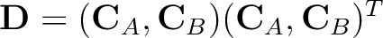 where
where  is the corresponding canonical
MOs matrix for the state A and B.
When computing the coupling between 2 different
states A and B, only for the first state we use pure Cholesky MOs. The invariance of the Fock matrix
is then ensured by rotating the orbitals of B according to the orthogonal matrix defined in A
through the Cholesky localization. These orbitals used for B are therefore called ``pseudo Cholesky MOs''.
is the corresponding canonical
MOs matrix for the state A and B.
When computing the coupling between 2 different
states A and B, only for the first state we use pure Cholesky MOs. The invariance of the Fock matrix
is then ensured by rotating the orbitals of B according to the orthogonal matrix defined in A
through the Cholesky localization. These orbitals used for B are therefore called ``pseudo Cholesky MOs''.
8.42.3.2 Input example
»COPY "Jobiph file 1" JOB001 »COPY "Jobiph file 2" JOB002 »COPY "Jobiph file 3" JOB003&RASSI
NR OF JOBIPHS= 3 4 2 2 -- 3 JOBIPHs. Nr of states from each.
1 2 3 4; 3 4; 3 4 -- Which roots from each JOBIPH.
CIPR; THRS= 0.02
Properties= 4; 'MltPl 1' 1 'MltPl 1' 3 'Velocity' 1 'Velocity' 3
* This input will compute eigenstates in the space
* spanned by the 8 input functions. Assume only the first
* 4 are of interest, and we want natural orbitals out
NATO= 4
Next: 8.43 rpa Up: 8. Programs Previous: 8.41 rasscf