MOLCAS manual:

Next: 10.3 Computing a reaction path.
Up: 10. Examples
Previous: 10.1 Computing high symmetry molecules.
Subsections
10.2 Geometry optimizations and Hessians.
To optimize a molecular geometry is probably one of the most frequent
interests of a quantum chemist [247]. In the present section we examine
some examples of obtaining stationary points on the energy surfaces.
We will focus in this section in searching of minimal energy points,
postponing the discussion on transition states to section ![[*]](crossref.png) .
This type of calculations require the computation of molecular gradients,
whether using analytical or numerical derivatives. We will also examine
how to obtain the full geometrical Hessian for a molecular state, what
will provide us with vibrational frequencies within the harmonic
approximation and thermodynamic properties by the use of the proper
partition functions. .
This type of calculations require the computation of molecular gradients,
whether using analytical or numerical derivatives. We will also examine
how to obtain the full geometrical Hessian for a molecular state, what
will provide us with vibrational frequencies within the harmonic
approximation and thermodynamic properties by the use of the proper
partition functions.
The program ALASKA computes analytical gradients for optimized wave
functions. In 8.1 the SCF, DFT, and CASSCF/RASSCF levels of calculation are
available. The program ALASKA also computes numerical gradients
from CASPT2 and MS-CASPT2 energies. Provided with the first order derivative matrix with respect to the
nuclei and an approximate guess of the Hessian matrix, the program
SLAPAF is then used to optimize molecular structures. From MOLCAS-5 it is
not necessary to explicitly define the set of internal coordinates
of the molecule in the SLAPAF input. Instead a redundant coordinates
approach is used. If the definition is absent
the program builds its own set of parameters based on
curvature-weighted non-redundant internal coordinates and displacements
[161]. As they depend
on the symmetry of the system it might be somewhat difficult in some
systems to define them. It is, therefore, strongly recommended to let
the program define its own set of non-redundant internal coordinates.
In certain situations such as bond dissociations the previous coordinates
may not be appropriate and the code directs the user to use instead
Cartesian coordinates, for instance.
As an example we are going to work with the 1,3-cyclopentadiene
molecule. This is a five-carbon system forming a ring which has
two conjugated double bonds. Each carbon has one attached
hydrogen atom except one which has two. We will use the
CASSCF method and
take advantage of the symmetry properties of the molecule to
compute ground and excited states. To ensure
the convergence of the results we will also perform
Hessian calculations to compute the force fields at the
optimized geometries.
In this section we will combine two types of procedures to perform
calculations in MOLCAS. The user may then choose the most convenient
for her/his taste. We can use an general script and perform an input-oriented
calculation, when all the information relative to the calculation, including
links for the files and control of iterations, are inserted in the input
file. The other procedure is the classical script-oriented system used in
previous examples and typically previous versions of MOLCAS. Let's start
by making an input-oriented optimization. A script is still needed to
perform the basic definitions, although they can be mostly done within the
input file. A suggested form for this general script could be:
#!/bin/sh
export MOLCAS=/home/molcas/molcashome
export MOLCAS_MEM=64
export Project=Cyclopentadiene1
export HomeDir=/home/somebody/somewhere
export WorkDir=$HomeDir/$Project
[ ! -d $WorkDir ] && mkdir $WorkDir
molcas $HomeDir/$Project.input >$HomeDir/$Project.out 2>$HomeDir/$Project.err
exit
We begin by defining the input for the initial calculation.
In simple cases the optimization procedure is very efficient.
We are going, however, to design a more complete procedure that
may help in more complex situations.
It is sometimes useful to start the optimization in a small
size basis set and use the obtained approximate Hessian to
continue the calculation with larger basis sets. Therefore,
we will begin by using the minimal STO-3G basis set to optimize
the ground state of 1,3-cyclopentadiene within C2v symmetry.
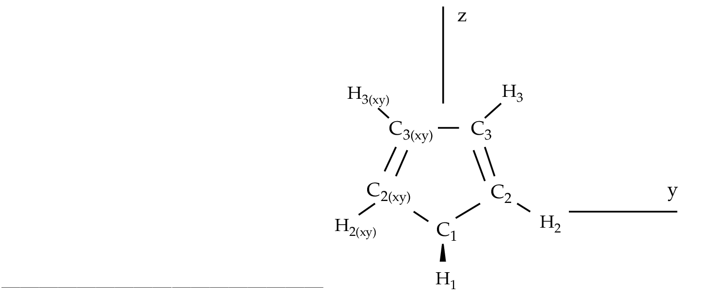
Figure 10.2:
1,3-cyclopentadiene
 |
>>> EXPORT MOLCAS_MAXITER=50
&GATEWAY; Title=1,3,-cyclopentadiene. STO-3G basis set.
Symmetry= X XY
Basis set
C.STO-3G....
C1 0.000000 0.000000 0.000000 Bohr
C2 0.000000 2.222644 1.774314 Bohr
C3 0.000000 1.384460 4.167793 Bohr
End of basis
Basis set
H.STO-3G....
H1 1.662033 0.000000 -1.245623 Bohr
H2 0.000000 4.167844 1.149778 Bohr
H3 0.000000 2.548637 5.849078 Bohr
End of basis
>>> Do while <<<
&SEWARD
>>> IF ( ITER = 1 )
&SCF
TITLE= cyclopentadiene molecule
OCCUPIED=9 1 6 2
ITERATIONS=40
>>> END IF
&RASSCF
TITLE=cyclopentadiene molecule 1A1
SYMMETRY=1; SPIN=1
NACTEL= 6 0 0
INACTIVE= 9 0 6 0
RAS2= 0 2 0 3 <--- All pi valence orbitals active
ITER= 50,25; CIMX= 25
&ALASKA
&SLAPAF; Iterations=80; Thrs=0.5D-06 1.0D-03
>>> EndDo <<<
>>> COPY $Project.RunFile $CurrDir/$Project.ForceConstant.STO-3G
A copy of the RUNFILE has been made at the end of the input stream.
This saves the file for use as (a) starting geometry and (b)
a guess of the Hessian matrix in the following calculation.
The link can be also done in the shell
script.
The generators used to define the
C2v symmetry are X and XY, plane yz and axis z. They
differ from those used in other examples as in section .
The only consequence is that the order of the symmetries in SEWARD
differs. In the present case the order is:  , ,  , ,  , and , and  ,
and consequently the classification by symmetries of the orbitals
in the SCF and RASSCF inputs will differ. It is therefore
recommended to initially use the option TEST in the GATEWAY input
to check the symmetry option. This option, however, will stop the calculation
after the GATEWAY input head is printed. ,
and consequently the classification by symmetries of the orbitals
in the SCF and RASSCF inputs will differ. It is therefore
recommended to initially use the option TEST in the GATEWAY input
to check the symmetry option. This option, however, will stop the calculation
after the GATEWAY input head is printed.
The calculation converges in four steps. We change now the input. We can
choose between replacing by hand the geometry of the SEWARD input
or use the same $WorkDir directory and let the program to take the last
geometry stored into the RUNFILE file. In any case the
new input can be:
>>COPY $CurrDir/OPT.hessian.ForceConstant.STO-3G $Project.RunOld
&GATEWAY; Title=1,3,-cyclopentadiene molecule
Symmetry=X XY
Basis set
C.ANO-L...4s3p1d.
C1 .0000000000 .0000000000 -2.3726116671
C2 .0000000000 2.2447443782 -.5623842095
C3 .0000000000 1.4008186026 1.8537195887
End of basis
Basis set
H.ANO-L...2s.
H1 1.6523486260 .0000000000 -3.6022531906
H2 .0000000000 4.1872267035 -1.1903003793
H3 .0000000000 2.5490335048 3.5419847446
End of basis
>>> Do while <<<
&SEWARD
>>> IF ( ITER = 1 ) <<<<
&SCF
TITLE=cyclopentadiene molecule
OCCUPIED= 9 1 6 2
ITERATIONS= 40
>>> ENDIF <<<
&RASSCF; TITLE cyclopentadiene molecule 1A1
SYMMETRY=1; SPIN=1; NACTEL=6 0 0
INACTIVE= 9 0 6 0
RAS2 = 0 2 0 3
ITER=50,25; CIMX= 25
&SLAPAF; Iterations=80; Thrs=0.5D-06 1.0D-03
OldForce Constant Matrix
>>> EndDo <<<
The RUNOLD file will be used by SEWARD to pick up
the molecular structure on the initial iteration and
by SLAPAF as initial Hessian
to carry out the relaxation. This use of the RUNFILE can be
done between any different calculations provided they work in the
same symmetry.
In the new basis set, the resulting
optimized geometry at the CASSCF level in C2v symmetry is:
********************************************
* Values of internal coordinates *
********************************************
C2C1 2.851490 Bohr
C3C2 2.545737 Bohr
C3C3 2.790329 Bohr
H1C1 2.064352 Bohr
H2C2 2.031679 Bohr
H3C3 2.032530 Bohr
C1C2C3 109.71 Degrees
C1C2H2 123.72 Degrees
C2C3H3 126.36 Degrees
H1C1H1 107.05 Degrees
Once we have the optimized geometry we can obtain the
force field, to compute the force constant matrix and
obtain an analysis of the harmonic frequency. This is done by
computing the analytical Hessian at the optimized geometry.
Notice that this is a single-shot calculation using the
MCKINLEY, which will automatically start the MCLR module
in case of a frequency calculation.
&GATEWAY; Title=1,3,-cyclopentadiene molecule
Symmetry= X XY
Basis set
C.ANO-L...4s3p1d.
C1 0.0000000000 0.0000000000 -2.3483061484
C2 0.0000000000 2.2245383122 -0.5643712787
C3 0.0000000000 1.3951643642 1.8424767578
End of basis
Basis set
H.ANO-L...2s.
H1 1.6599988023 0.0000000000 -3.5754797471
H2 0.0000000000 4.1615845660 -1.1772096132
H3 0.0000000000 2.5501642966 3.5149458446
End of basis
&SEWARD
&SCF; TITLE=cyclopentadiene molecule
OCCUPIED= 9 1 6 2
ITERATIONS= 40
&RASSCF; TITLE=cyclopentadiene molecule 1A1
SYMMETRY=1; SPIN=1; NACTEL= 6 0 0
INACTIVE= 9 0 6 0
RAS2 = 0 2 0 3
ITER= 50,25; CIMX=25
&MCKINLEY
Cyclopentadiene has 11 atoms, that mean 3N = 33 Cartesian degrees of freedom.
Therefore the MCLR output will contain 33 frequencies. From those,
we are just interested in the 3N-6 = 27 final degrees of freedom that
correspond to the normal modes of the system. We will discard from the
output the three translational (Ti) and three rotational (Ri) coordinates.
The table of characters gives us the classification of these six coordinates:
a1 (Tz), a2 (Rz), b2 (Tx,Ry), b1 (Ty,Rx).
This information is found in the Seward output:
Character Table for C2v
E s(yz) C2(z) s(xz)
a1 1 1 1 1 z
a2 1 -1 1 -1 xy, Rz, I
b2 1 1 -1 -1 y, yz, Rx
b1 1 -1 -1 1 x, xz, Ry
It is simply to distinguish these frequencies because they must be zero,
although and because of numerical inaccuracies they will be simply close
to zero. Note that the associated intensities are nonsense.
In the present calculation the harmonic frequencies, the infrared
intensities, and the corresponding normal modes printed below in Cartesian
coordinates are the following:
Symmetry a1
==============
1 2 3 4 5 6
Freq. 0.04 847.85 966.08 1044.69 1187.61 1492.42
Intensity: 0.646E-08 0.125E-02 0.532E+01 0.416E+00 0.639E-01 0.393E+01
C1 z 0.30151 0.35189 -0.21166 -0.11594 0.06874 0.03291
C2 y 0.00000 0.31310 0.14169 0.12527 -0.01998 -0.08028
C2 z 0.30151 -0.02858 0.06838 -0.00260 0.02502 -0.06133
C3 y -0.00000 0.04392 -0.07031 0.23891 -0.02473 0.16107
C3 z 0.30151 -0.15907 0.00312 0.08851 -0.07733 -0.03146
H1 x 0.00000 -0.02843 -0.00113 -0.01161 0.00294 0.04942
H1 z 0.30151 0.31164 -0.21378 -0.13696 0.08233 0.11717
H2 y 0.00000 0.24416 0.27642 0.12400 0.11727 0.07948
H2 z 0.30151 -0.25054 0.46616 -0.05986 0.47744 0.46022
H3 y -0.00000 -0.29253 -0.28984 0.59698 0.34878 -0.34364
H3 z 0.30151 0.07820 0.15644 -0.13576 -0.34625 0.33157
7 8 9 10 11
Freq. 1579.76 1633.36 3140.69 3315.46 3341.28
Intensity: 0.474E+01 0.432E+00 0.255E+02 0.143E+02 0.572E+01
...
Symmetry a2
==============
1 2 3 4 5
Freq. i9.26 492.62 663.74 872.47 1235.06
...
Symmetry b2
==============
1 2 3 4 5 6
Freq. i10.61 0.04 858.72 1020.51 1173.33 1386.20
Intensity: 0.249E-01 0.215E-07 0.259E+01 0.743E+01 0.629E-01 0.162E+00
...
7 8 9 10
Freq. 1424.11 1699.07 3305.26 3334.09
Intensity: 0.966E+00 0.426E+00 0.150E+00 0.302E+02
...
Symmetry b1
==============
1 2 3 4 5 6
Freq. i11.31 0.11 349.15 662.98 881.19 980.54
Intensity: 0.459E-01 0.202E-06 0.505E+01 0.896E+02 0.302E+00 0.169E+02
...
7
Freq. 3159.81
Intensity: 0.149E+02
...
Apart from the six mentioned translational and rotational coordinates
There are no imaginary frequencies and therefore the geometry corresponds
to a stationary point within the C2v symmetry.
The frequencies are expressed in reciprocal centimeters.
After the vibrational analysis the zero-point energy correction and the thermal
corrections to the total energy, internal, entropy, and Gibbs free energy.
The analysis uses the standard expressions for an ideal gas in the canonical
ensemble which can be found in any standard statistical mechanics book.
The analysis is performed at different temperatures, for instance:
*****************************************************
Temperature = 273.00 Kelvin, Pressure = 1.00 atm
-----------------------------------------------------
Molecular Partition Function and Molar Entropy:
q/V (M**-3) S(kcal/mol*K)
Electronic 0.100000D+01 0.000
Translational 0.143889D+29 38.044
Rotational 0.441593D+05 24.235
Vibrational 0.111128D-47 3.002
TOTAL 0.706112D-15 65.281
Thermal contributions to INTERNAL ENERGY:
Electronic 0.000 kcal/mol 0.000000 au.
Translational 0.814 kcal/mol 0.001297 au.
Rotational 0.814 kcal/mol 0.001297 au.
Vibrational 60.723 kcal/mol 0.096768 au.
TOTAL 62.350 kcal/mol 0.099361 au.
Thermal contributions to
ENTHALPY 62.893 kcal/mol 0.100226 au.
GIBBS FREE ENERGY 45.071 kcal/mol 0.071825 au.
Sum of energy and thermal contributions
INTERNAL ENERGY -192.786695 au.
ENTHALPY -192.785831 au.
GIBBS FREE ENERGY -192.814232 au.
Next, polarizabilities (see below) and isotope shifted frequencies are also displayed
in the output.
************************************
* *
* Polarizabilities *
* *
************************************
34.76247619
-0.00000000 51.86439359
-0.00000000 -0.00000000 57.75391824
For a graphical representation of the harmonic frequencies one can also use the
$Project.freq.molden file as an input to the MOLDEN program.
The calculation of excited states using the ALASKA and SLAPAF codes
has no special characteristic. The wave function is defined by the
SCF or RASSCF programs. Therefore if we want to optimize an excited
state the RASSCF input has to be defined accordingly. It is not,
however, an easy task, normally because the excited states have lower
symmetry than the ground state and one has to work in low order
symmetries if the full optimization is pursued.
Take the example of the thiophene molecule (see fig.
in next section). The ground state has
C2v symmetry: 1 1A1. The two lowest valence excited states
are 21A1 and 11B2. If we optimize the geometries within
the C2v symmetry the calculations converge easily for the three
states. They are the first, second, and first roots of their
symmetry, respectively. But if we want to make a full optimization
in C1, or even a restricted one in Cs, all three states belong
to the same symmetry representation. The higher the root more
difficult is to converge it. A geometry optimization requires
single-root optimized CASSCF wave-functions, but, unlike in previous MOLCAS versions, we can now carry out State-Average (SA) CASSCF calculations
between different roots. The wave functions we have with this procedure
are based on an averaged density matrix, and a further orbital relaxation
is required. The MCLR program can perform such a task by means
of a perturbational approach. Therefore, if we choose to carry out a
SA-CASSCF calculations in the optimization procedure, the Alaska
module will automatically start up the MCLR module.
We are going to optimize the three states of thiophene in C2v symmetry. The inputs are:
&GATEWAY; Title=Thiophene molecule
Symmetry= X XY
Basis set
S.ANO-S...4s3p2d.
S1 .0000000000 .0000000000 -2.1793919255
End of basis
Basis set
C.ANO-S...3s2p1d.
C1 .0000000000 2.3420838459 .1014908659
C2 .0000000000 1.3629012233 2.4874875281
End of basis
Basis set
H.ANO-S...2s.
H1 .0000000000 4.3076765963 -.4350463731
H2 .0000000000 2.5065969281 4.1778544652
End of basis
>>> Do while <<<
&SEWARD
>>> IF ( ITER = 1 ) <<<
&SCF; TITLE=Thiophene molecule
OCCUPIED= 11 1 7 3
ITERATIONS= 40
>>> ENDIF <<<
&RASSCF; TITLE=Thiophene molecule 1 1A1
SYMMETRY=1; SPIN=1; NACTEL= 6 0 0
INACTIVE= 11 0 7 1
RAS2 = 0 2 0 3
ITER= 50,25
&ALASKA
&SLAPAF
End of Input
>>> ENDDO <<<
for the ground state. For the two excited states we will replace
the RASSCF inputs with
&RASSCF; TITLE=Thiophene molecule 2 1A1
SYMMETRY=1; SPIN=1; NACTEL= 6 0 0
INACTIVE= 11 0 7 1
RAS2 = 0 2 0 3
ITER= 50,25
CIROOT= 2 2; 1 2; 1 1
LEVSHFT=1.0
RLXRoot= 2
for the 21A1 state.
Notice that we are doing a SA-CASSCF calculation
including two roots, therefore we must use
the keyword RLXROOT within the RASSCF input
to specify for which state we want the root.
We have also
&RASSCF; TITLE=Thiophene molecule 1 1B2
SYMMETRY=2; SPIN=1; NACTEL= 6 0 0
INACTIVE= 11 0 7 1
RAS2 = 0 2 0 3
ITER= 50,25
LEVSHFT=1.0
for the 11B2 state.
To help the program to converge we can include one or more initial RASSCF
inputs in the input file.
The following is an example for the calculation
of the of the 31A' state of thiophene (Cs symmetry) with a previous
calculation of the ground state to have better starting orbitals.
&GATEWAY; Title= Thiophene molecule
Symmetry=X
Basis set
S.ANO-S...4s3p2d.
S1 .0000000000 .0000000000 -2.1174458547
End of basis
Basis set
C.ANO-S...3s2p1d.
C1 .0000000000 2.4102089951 .1119410701
C1b .0000000000 -2.4102089951 .1119410701
C2 .0000000000 1.3751924147 2.7088559532
C2b .0000000000 -1.3751924147 2.7088559532
End of basis
Basis set
H.ANO-S...2s.
H1 .0000000000 4.3643321746 -.4429940876
H1b .0000000000 -4.3643321746 -.4429940876
H2 .0000000000 2.5331491787 4.3818833166
H2b .0000000000 -2.5331491787 4.3818833166
End of basis
>>> Do while <<<
&SEWARD
>>> IF ( ITER = 1 ) <<<
&SCF; TITLE= Thiophene molecule
OCCUPIED= 18 4
ITERATIONS = 40
&RASSCF; TITLE= Thiophene molecule 1A'
SYMMETRY=1; SPIN=1; NACTEL= 6 0 0
INACTIVE= 18 1
RAS2 = 0 5
ITER= 50,25
>>> ENDIF <<<
&RASSCF; TITLE= Thiophene molecule 3 1A'
SYMMETRY=1; SPIN=1; NACTEL= 6 0 0
INACTIVE= 18 1
RAS2 = 0 5
ITER= 50,25
CIROOT=3 3 1
RLXRoot= 3
&ALASKA
&SLAPAF &END
>>> ENDDO <<<
It should be remembered that geometry optimizations for excited states
are difficult. Not only can it be difficult to converge the corresponding
RASSCF calculation, but we must also be sure that the order of the
states does not change during the optimization of the geometry. This is
not uncommon and the optimization must be followed by the user.
10.2.3.1 Optimizing with geometrical constraints.
A common situation in geometry optimizations is to have one or
several coordinates fixed or constrained and vary the remaining coordinates.
As an example we will take the biphenyl molecule, two benzene moieties
bridged by a single bond. The ground state of the molecule is not
planar. One benzene group is twisted by 44 degrees with
respect to the other [248]. We can use this example to perform
two types of restricted optimizations. The simplest way to introduce
constraints is to give a coordinate a fixed value and let the other
coordinates to be optimized. For instance, let's fix the dihedral
angle between both benzenes to be fixed to 44 degrees. Within
this restriction, the remaining coordinates will be fully optimized.
The Constraints keyword in the program GATEWAY will
take care of the restriction (note this keyword could also
be placed in the program SLAPAF). The input could be: degrees with
respect to the other [248]. We can use this example to perform
two types of restricted optimizations. The simplest way to introduce
constraints is to give a coordinate a fixed value and let the other
coordinates to be optimized. For instance, let's fix the dihedral
angle between both benzenes to be fixed to 44 degrees. Within
this restriction, the remaining coordinates will be fully optimized.
The Constraints keyword in the program GATEWAY will
take care of the restriction (note this keyword could also
be placed in the program SLAPAF). The input could be:
&GATEWAY; Title= Biphenyl twisted D2
Symmetry= XY XZ
Basis set
C.ANO-S...3s2p1d.
C1 1.4097582886 .0000000000 .0000000000
C2 2.7703009377 2.1131321616 .8552434921
C3 5.4130377085 2.1172148045 .8532344474
C4 6.7468359904 .0000000000 .0000000000
End of basis
Basis set
H.ANO-S...2s.
H2 1.7692261798 3.7578798540 1.5134152112
H3 6.4188773347 3.7589592975 1.5142479153
H4 8.7821560635 .0000000000 .0000000000
End of basis
Constraints
d1 = Dihedral C2 C1 C1(XY) C2(XY)
Values
d1 = -44.4 degrees
End of Constraints
>>> Do while <<<
&SEWARD
>>> IF ( ITER = 1 ) <<<
&SCF; TITLE= Biphenyl twisted D2
OCCUPIED= 12 9 9 11
ITERATIONS= 50
>>> ENDIF <<<
&RASSCF; TITLE= Biphenyl twisted D2
SYMMETRY=1; SPIN=1; NACTEL= 12 0 0
INACTIVE= 11 7 7 10
RAS2 = 2 4 4 2
&ALASKA
&SLAPAF; Iterations=30; MaxStep=1.0
>>> ENDDO <<<
One important consideration about the constraint. You do not need
to start at a geometry having the exact value for the coordinate
you have selected (44.4 degrees for the dihedral angle here).
The optimization will lead you to the right solution. On the other
hand, if you start exactly with the dihedral being 44.4 deg the
code does not necessarily will freeze this value in the first
iterations, but will converge to it at the end. Therefore, it may
happen that the value for the dihedral differs from the selected
value in the initial iterations. You can follow the optimization
steps in the $WorkDir directory using the MOLDEN files generated
automatically by MOLCAS.
Now we will perform the opposite optimization: we want to optimize the
dihedral angle relating both benzene units but keep all the other
coordinates fixed. We could well use the same procedure as before
adding constraints for all the remaining coordinates different from
the interesting dihedral angle, but to build the input would be
tedious. Therefore, instead of keyword Constraints we
will make use of the keywords Vary and Fix.
The input file should be:
&GATEWAY; Title= Biphenyl twisted D2
Symmetry=XY XZ
Basis set
C.ANO-S...3s2p1d.
C1 1.4097582886 .0000000000 .0000000000
C2 2.7703009377 2.1131321616 .8552434921
C3 5.4130377085 2.1172148045 .8532344474
C4 6.7468359904 .0000000000 .0000000000
End of basis
Basis set
H.ANO-S...2s.
H2 1.7692261798 3.7578798540 1.5134152112
H3 6.4188773347 3.7589592975 1.5142479153
H4 8.7821560635 .0000000000 .0000000000
End of basis
>>> Do while <<<
&SEWARD
>>> IF ( ITER = 1 ) <<<
&SCF; TITLE= Biphenyl twisted D2
OCCUPIED= 12 9 9 11
ITERATIONS= 50
>>> ENDIF <<<
&RASSCF; TITLE= Biphenyl twisted D2
SYMMETRY=1; SPIN=1; NACTEL=12 0 0
INACTIVE= 11 7 7 10
RAS2 = 2 4 4 2
&ALASKA
&SLAPAF
Internal coordinates
b1 = Bond C1 C1(XY)
b2 = Bond C1 C2
b3 = Bond C2 C3
b4 = Bond C3 C4
h1 = Bond C2 H2
h2 = Bond C3 H3
h3 = Bond C4 H4
a1 = Angle C2 C1 C1(XY)
a2 = Angle C1 C2 C3
a3 = Angle C1 C2 H2
a4 = Angle C2 C3 H3
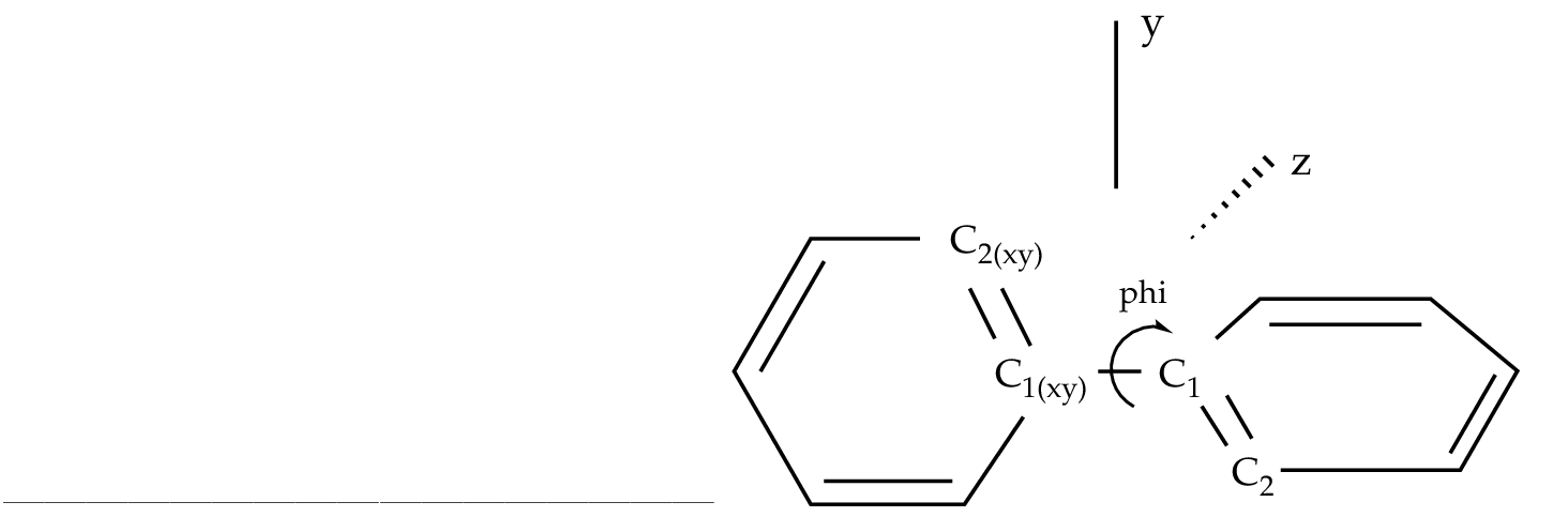
phi = Dihedral C2 C1 C1(XY) C2(XY)
d1 = Dihedral H2 C2 C1 C1(XY)
d2 = OutOfP C3 C1(XY) C1 C2
d3 = Dihedral H3 C3 C2 H2
Vary; phi
Fix; b1; b2; b3; b4; h1; h2; h3; a1; a2; a3; a4; d1; d2; d3
End of Internal
Iterations= 30
>>> ENDDO <<<
To be able to optimize the molecule in that way a D2 symmetry
has to be used. In the definition of the internal coordinates
we can use an out-of-plane coordinate: C2 C2(xy) C1(xy) C1 or
a dihedral angle
C2 C1 C1(xy) C2(xy). In this case there is no major problem but
in general one has to avoid as much as possible to define
dihedral angles close to 180 ( trans conformation ).
The SLAPAF program will warn about this problem if necessary.
In the present example, angle 'phi' is the angle to vary
while the remaining coordinates are frozen. All this is only
a problem in the user-defined internal approach, not in the
non-redundant internal approach used by default in the program.
In case we do not have the coordinates from a previous calculation
we can always run a simple calculation with one iteration
in the SLAPAF program.
It is not unusual to have problems in the relaxation step when
one defines internal coordinates. Once the program has found that
the definition is consistent with the molecule and the symmetry,
it can happen that the selected coordinates are not the best choice
to carry out the optimization, that the variation of some of the
coordinates is too large or maybe some of the angles are close
to their limiting values ( 180 for Dihedral angles and
90 for Out of Plane angles). The SLAPAF program will
inform about these problems. Most of the situations are solved by
re-defining the coordinates, changing the basis set or the geometry
if possible, or even freezing some of the coordinates.
One easy solution is to froze this particular coordinate and optimize,
at least partially, the other as an initial step to a full
optimization. It can be recommended to change the definition of the
coordinates from internal to Cartesian. 180 for Dihedral angles and
90 for Out of Plane angles). The SLAPAF program will
inform about these problems. Most of the situations are solved by
re-defining the coordinates, changing the basis set or the geometry
if possible, or even freezing some of the coordinates.
One easy solution is to froze this particular coordinate and optimize,
at least partially, the other as an initial step to a full
optimization. It can be recommended to change the definition of the
coordinates from internal to Cartesian.
Figure 10.3:
Twisted biphenyl molecule
 |
10.2.3.2 Optimizing with symmetry restrictions.
Presently, MOLCAS is prepared to work in the point groups
C1, Ci, Cs, C2, D2, C2h, C2v, and D2h.
To have the wave functions or geometries in other symmetries we
have to restrict orbital rotations or geometry relaxations specifically.
We have shown how to in the RASSCF program by using the
SUPSym option. In a geometry optimization we may also want to
restrict the geometry of the molecule to other symmetries. For
instance, to optimize the benzene molecule which belongs to the
D6h point group we have to generate the integrals and
wave function in D2h symmetry, the highest group available,
and then make the appropriate combinations of the coordinates
chosen for the relaxation in the SLAPAF program, as is shown
in the manual.
As an example we will take the ammonia molecule, NH3. There is
a planar transition state along the isomerization barrier between
two pyramidal structures. We want to optimize the planar structure
restricted to the D3h point group. However, the electronic wave function will
be computed in Cs symmetry (C2v is also possible)
and will not be restricted, although it is possible to do that
in the RASSCF program.
The input for such a geometry optimization is:
&GATEWAY; Title= NH3, planar
Symmetry= Z
Basis Set
N.ANO-L...4s3p2d.
N .0000000000 .0000000000 .0000000000
End of Basis
Basis set
H.ANO-L...3s2p.
H1 1.9520879910 .0000000000 .0000000000
H2 -.9760439955 1.6905577906 .0000000000
H3 -.9760439955 -1.6905577906 .0000000000
End of Basis
>>> Do while <<<
&SEWARD
>>> IF ( ITER = 1 ) <<<
&SCF; Title= NH3, planar
Occupied= 4 1
Iterations= 40
>>> ENDIF <<<
&RASSCF; Title= NH3, planar
Symmetry=1; Spin=1; Nactel=8 0 0
INACTIVE=1 0
RAS2 =6 2
&ALASKA
&SLAPAF
Internal coordinates
b1 = Bond N H1
b2 = Bond N H2
b3 = Bond N H3
a1 = Angle H1 N H2
a2 = Angle H1 N H3
Vary
r1 = 1.0 b1 + 1.0 b2 + 1.0 b3
Fix
r2 = 1.0 b1 - 1.0 b2
r3 = 1.0 b1 - 1.0 b3
a1 = 1.0 a1
a2 = 1.0 a2
End of internal
>>> ENDDO <<<
All four atoms are in the same plane.
Working in Cs, planar ammonia has five degrees of freedom.
Therefore we must define five independent internal coordinates, in this
case the three N-H bonds and two of the three angles H-N-H. The
other is already defined knowing the two other angles.
Now we must define the varying coordinates. The bond lengths will
be optimized, but all three N-H distances must be equal.
First we define (see definition in the previous input)
coordinate r1 equal to the sum of all three
bonds; then, we define coordinates r2 and r3 and keep them fixed.
r2 will ensure that bond1 is equal to bond2 and r3 will assure that
bond3 is equal to bond1. r2 and r3 will have a zero value.
In this way all three bonds will have the same length.
As we want the system constrained into the D3h point group,
the three angles must be equal with a value of 120 degrees. This is
their initial value, therefore we simply keep coordinates ang1 and ang2
fixed. The result is a D3h structure:
*******************************************
* InterNuclear Distances / Angstrom *
*******************************************
1 N 2 H1 3 H2 4 H3
1 N 0.000000
2 H1 1.003163 0.000000
3 H2 1.003163 1.737529 0.000000
4 H3 1.003163 1.737529 1.737529 0.000000
**************************************
* Valence Bond Angles / Degree *
**************************************
Atom centers Phi
2 H1 1 N 3 H2 120.00
2 H1 1 N 4 H3 120.00
3 H2 1 N 4 H3 120.00
In a simple case like this an optimization without
restrictions would also end up in the same symmetry as the initial
input.
10.2.4 Optimizing with Z-Matrix.
An alternative way to optimize a structure with geometrical and/or symmetrical
constraints is to combine the Z-Matrix definition of the molecular structure
used for the program SEWARD with a coherent definition for the
Internal Coordinated used in the optimization by program SLAPAF.
Here is an examples of optimization of the methyl carbanion. Note that the
wavefunction is calculated within the Cs symmetry but the geometry is optimized
within the C3v symmetry through the ZMAT and the Internal
Coordinates definitions. Note that XBAS precedes ZMAT.
&Gateway
Symmetry=Y
XBAS=Aug-cc-pVDZ
ZMAT
C1
X2 1 1.00
H3 1 1.09 2 105.
H4 1 1.09 2 105. 3 120.
>>> export MOLCAS_MAXITER=500
>>> Do While <<<
&SEWARD
&SCF; Charge= -1
&ALASKA
&SLAPAF
Internal Coordinates
CX2 = Bond C1 X2
CH3 = Bond C1 H3
CH4 = Bond C1 H4
XCH3 = Angle X2 C1 H3
XCH4 = Angle X2 C1 H4
DH4 = Dihedral H3 X2 C1 H4
Vary
SumCH34 = 1. CH3 +2. CH4
SumXCH34 = 1. XCH3 +2. XCH4
Fix
rCX2 = 1.0 CX2
DifCH34 = 2. CH3 -1. CH4
DifXCH34 = 2. XCH3 -1. XCH4
dDH4 = 1.0 DH4
End of Internal
PRFC
Iterations= 10
>>> EndDo <<<
Note that the dummy atom X2 is used to define the Z axis and the planar angles
for the hydrogen atoms. The linear combinations of bond distances and planar
angles in the expression in the Vary and Fix sections are used
to impose the C3v symmetry.
Another examples where the wavefunction and the geometry can be calculated
within different symmetry groups is benzene. In this case, the former uses
D2h symmetry and the latter D6h symmetry. Two special atoms are
used: the dummy X1 atom defines the center of the molecule while the ghost
Z2 atom is used to define the C6 rotational axis (and the Z axis).
&GATEWAY
Symmetry=X Y Z
XBAS
H.ANO-S...2s.
C.ANO-S...3s2p.
End of basis
ZMAT
X1
Z2 1 1.00
C3 1 1.3915 2 90.
C4 1 1.3915 2 90. 3 60.
H5 1 2.4715 2 90. 3 0.
H6 1 2.4715 2 90. 3 60.
>>> export MOLCAS_MAXITER=500
>>> Do While <<<
&SEWARD; &SCF ; &ALASKA
&SLAPAF
Internal Coordinates
XC3 = Bond X1 C3
XC4 = Bond X1 C4
XH5 = Bond X1 H5
XH6 = Bond X1 H6
CXC = Angle C3 X1 C4
HXH = Angle H5 X1 H6
Vary
SumC = 1.0 XC3 + 2.0 XC4
SumH = 1.0 XH5 + 2.0 XH6
Fix
DifC = 2.0 XC3 - 1.0 XC4
DifH = 2.0 XH5 - 1.0 XH6
aCXC = 1.0 CXC
aHXH = 1.0 HXH
End of Internal
PRFC
>>> EndDo <<<
Note that the ghost atom Z2 is used to define the geometry within the Z-Matrix
but it does not appear in the Internal Coordinates section. On the
other hand, the dummy atom X1 represents the center of the molecule and it
is used in the Internal Coordinates section.
10.2.5 CASPT2 optimizations
For systems showing a clear multiconfigurational nature, the CASSCF
treatment on top of the HF results is of crucial importance in order to
recover the large non dynamical correlation effects.
On the other hand, ground-state geometry optimizations of closed
shell systems are not exempt from non dynamical correlation effects.
In general, molecules containing  -electrons suffer from significant
effects of non dynamical correlation, even more in presence of
conjugated groups. Several studies on systems with delocalized bonds
have shown the effectiveness of the CASSCF approach in reproducing
the main geometrical parameters with
high accuracy [249,250,251]. -electrons suffer from significant
effects of non dynamical correlation, even more in presence of
conjugated groups. Several studies on systems with delocalized bonds
have shown the effectiveness of the CASSCF approach in reproducing
the main geometrical parameters with
high accuracy [249,250,251].
However, pronounced effects of dynamical correlation often occur
in systems with -electrons, especially in combination with polarized
bonds. An example is given by the C=O bond length, which is known
to be very sensitive to an accurate
description of the dynamical correlation effects [252]. We will show now
that the inherent limitations of the CASSCF method can be successfully overcome by employing
a CASPT2 geometry optimization, which uses a numerical gradient procedure
of recent implementation. A suitable molecule for this investigation
is acrolein.
As many other conjugated aldehydes and ketones, offers an example
of s-cis/s-trans isomerism (Figure ). Due to the resonance
between various structures
involving electrons,
the bond order for the C-C bond is higher than the one for a non-conjugated
C-C single bond. This partial double-bond character restricts the rotation
about such a bond, giving rise to the possibility of geometrical isomerism,
analogue to the cis–trans one observed for conventional double bonds.
A CASPT2 geometry optimization can be performed in MOLCAS.
A possible input for the CASPT2 geometry optimization of the s-trans
isomer is displayed below. The procedure is invoking the resolution-of-identity
approximation using the keyword RICD. This option will speed up the
calculation, something which makes sense since we will compute the gradients numerically.
>>> Export MOLCAS_MAXITER=500
&GATEWAY
Title= Acrolein Cs symmetry - transoid
Coord
8
O 0.0000000 -1.4511781 -1.3744831
C 0.0000000 -0.8224882 -0.1546649
C 0.0000000 0.7589531 -0.0387200
C 0.0000000 1.3465057 1.2841925
H 0.0000000 -1.4247539 0.8878671
H 0.0000000 1.3958142 -1.0393956
H 0.0000000 0.6274048 2.2298215
H 0.0000000 2.5287634 1.4123985
Group=X
Basis=ANO-RCC-VDZP
RICD
>>>>>>>>>>>>> Do while <<<<<<<<<<<<
&SEWARD
>>>>>>>> IF ( ITER = 1 ) <<<<<<<<<<<
&SCF; Title= Acrolein Cs symmetry
*The symmetry species are a' a''
Occupied= 13 2
>>>>>>> ENDIF <<<<<<<<<<<<<<<<<<<<<
&RASSCF; Title=Acrolein ground state
nActEl= 4 0 0
Inactive= 13 0
* The symmetry species are a' a''
Ras2= 0 4
&CASPT2
&SLAPAF
>>>>>>>>>>>>> ENDDO <<<<<<<<<<<<<<
Experimental investigations assign a planar structure for both the
isomers. We can take advantage of this result and use a Cs symmetry
throughout the optimization procedure. Moreover, the choice of the
active space is suggested by previous calculations on analogous
systems. The active space contains 4 MOs /4 electrons, thus
what we will call shortly a -CASPT2 optimization.
The structure of the input follows the trends already explained in
other geometry optimizations, that is, loops over the set of programs
ending with SLAPAF. Notice that CASPT2 optimizations require
obviously the CASPT2 input, but also the input for the
ALASKA program, which computes the gradient numerically.
Apart from that, a CASPT2 optimization input is identical to the corresponding
CASSCF input.
One should note that the numerical gradients are not as accurate as the
analytic gradient. This can manifest itself in that there is no strict energy
lowering the last few iterations, as displayed below:
*****************************************************************************************************************
* Energy Statistics for Geometry Optimization *
*****************************************************************************************************************
Energy Grad Grad Step Estimated Geom Hessian
Iter Energy Change Norm Max Element Max Element Final Energy Update Update Index
1 -191.38831696 0.00000000 0.208203-0.185586 nrc007 -0.285508* nrc007 -191.41950985 RS-RFO None 0
2 -191.43810737 -0.04979041 0.117430-0.100908 nrc007 -0.190028* nrc007 -191.45424733 RS-RFO BFGS 0
3 -191.45332692 -0.01521954 0.022751-0.021369 nrc007 -0.051028 nrc007 -191.45399070 RS-RFO BFGS 0
4 -191.45414598 -0.00081906 0.012647 0.005657 nrc002 -0.013114 nrc007 -191.45421525 RS-RFO BFGS 0
5 -191.45422730 -0.00008132 0.003630 0.001588 nrc002 0.004050 nrc002 -191.45423299 RS-RFO BFGS 0
6 -191.45423140 -0.00000410 0.000744 0.000331 nrc006 0.000960 nrc013 -191.45423186 RS-RFO BFGS 0
7 -191.45423123 0.00000017 0.000208-0.000098 nrc003 -0.001107 nrc013 -191.45423159 RS-RFO BFGS 0
8 -191.45423116 0.00000007 0.000572 0.000184 nrc006 0.000422 nrc013 -191.45423131 RS-RFO BFGS 0
+----------------------------------+----------------------------------+
+ Cartesian Displacements + Gradient in internals +
+ Value Threshold Converged? + Value Threshold Converged? +
+-----+----------------------------------+----------------------------------+
+ RMS + 0.5275E-03 0.1200E-02 Yes + 0.1652E-03 0.3000E-03 Yes +
+-----+----------------------------------+----------------------------------+
+ Max + 0.7738E-03 0.1800E-02 Yes + 0.1842E-03 0.4500E-03 Yes +
+-----+----------------------------------+----------------------------------+
Geometry is converged in 8 iterations to a Minimum Structure
*****************************************************************************************************************
*****************************************************************************************************************
The calculation converges in 8 iterations. At this point it is worth noticing
how the convergence of CASPT2 energy is not chosen among the criteria for the
convergence of the structure. The final structure is in fact decided by checking the
Cartesian displacements and the gradient in non-redundant internal coordinates.
CASPT2 optimizations are expensive, however, the use for the resolution-of-identity
options gives some relife. Notice that they are based on numerical
gradients and many point-wise calculations are needed. In particular,
the Cartesian gradients are computed using a two-point formula.
Therefore, each macro-iteration
in the optimization requires 2*N + 1 Seward/RASSCF/CASPT2 calculations, with N being
the Cartesian degrees of freedom. In the present example, acrolein has eight atoms.
From each atom, only two Cartesian coordinates are free to move (we are working
within the Cs symmetry and the third coordinate is frozen), therefore the
total number of Seward/RASSCF/CASPT2 iterations within each macro-iteration
is 2*(8*2) + 1, that is, 33. In the current example a second trick has been
used to speed up the numerical calculation. The explicit reference to ALASKA
is excluded. This means that SLAPAF is called first without any gradients
beeing computed explicitly. It does then abort automatically requesting an implicit
calulation of the gradients, however, before doing so it compiles the internal coordinates
and sets up a list of displayed geometries to be used in a numerical gradient procedure.
In the present case this amounts to that the actuall number of micro iterations is
reduced from 33 to 29.
The Table displays the equilibrium geometrical
parameters computed at the -CASSCF and -CASPT2
level of theory
for the ground state of both isomers of acrolein. For sake of comparison,
Table includes
experimental data obtained from microwave spectroscopy
studies[253]. The computed parameters at -CASPT2 level are in
remarkable agreement with the experimental
data. The predicted value of the C=C bond length is very close to the double bond length
observed in ethylene. The other C-C bond has a length within the range expected
for a C-C single bond: it appears shorter in the s-trans isomer as a consequence
of the reduction of steric hindrance between the ethylenic and aldehydic
moieties. CASSCF estimates a carbon-oxygen bond length shorter
than the experimental value. For
-CASSCF optimization in conjugated systems this can be assumed as a general
behavior [254,252]. To explain such
a discrepancy, one may invoke the fact that the C=O bond distance is
particularly sensitive to electron correlation effects. The electron
correlation effects included at the -CASSCF level tend to overestimate bond
lengths. However, the lack of  electron correlation, goes
in the opposite direction, allowing shorter bond distances for double bonds.
For the C-C double bonds, these contrasting behaviors compensate each other
[251] resulting in quite an accurate value for the bond length at the
-CASSCF level. On the contrary, the extreme sensitivity of the C=O
bond length to the electron correlation effects, leads to a general
underestimation of the C-O double bond lengths, especially when such
a bond is part of a conjugated system. It is indeed the effectiveness of the CASPT2
method in recovering dynamical correlation which leads to a substantial improvement
in predicting the C-O double bond length. electron correlation, goes
in the opposite direction, allowing shorter bond distances for double bonds.
For the C-C double bonds, these contrasting behaviors compensate each other
[251] resulting in quite an accurate value for the bond length at the
-CASSCF level. On the contrary, the extreme sensitivity of the C=O
bond length to the electron correlation effects, leads to a general
underestimation of the C-O double bond lengths, especially when such
a bond is part of a conjugated system. It is indeed the effectiveness of the CASPT2
method in recovering dynamical correlation which leads to a substantial improvement
in predicting the C-O double bond length.

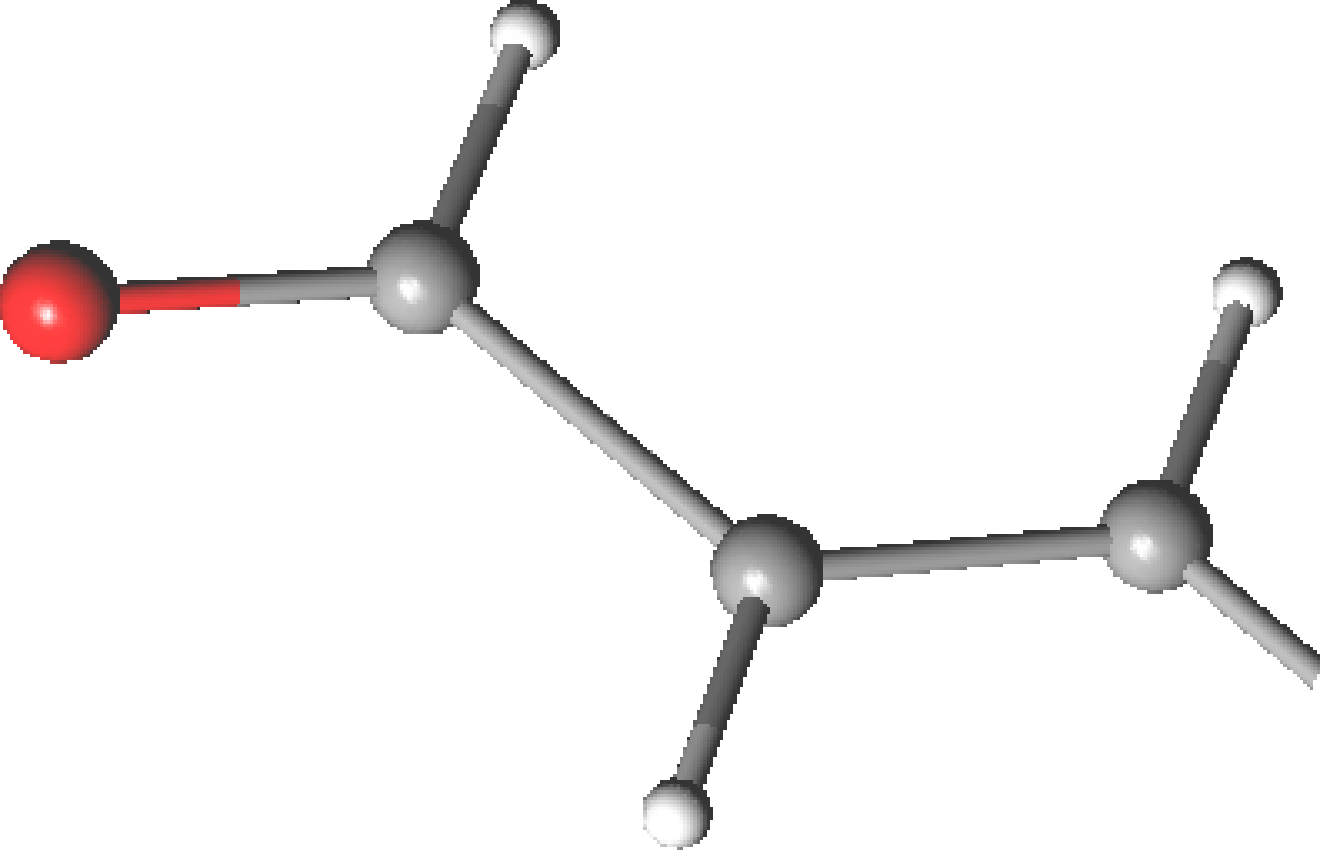
Table 10.8:
Geometrical parameters for the ground state of acrolein
| Parametersa |
-CASSCF [04/4] |
|
-CASPT2 |
|
Expt.b |
| |
s-cis |
s-trans |
|
s-cis |
s-trans |
|
|
| C1=O |
1.204 |
1.204 |
|
1.222 |
1.222 |
|
1.219 |
| C1–C2 |
1.483 |
1.474 |
|
1.478 |
1.467 |
|
1.470 |
| C2=C3 |
1.340 |
1.340 |
|
1.344 |
1.344 |
|
1.345 |
 C1C2C3 C1C2C3 |
123.0 |
121.7 |
|
121.9 |
120.5 |
|
119.8 |
| C2C1O |
124.4 |
123.5 |
|
124.5 |
124.2 |
|
- |
| aBond distances in Å and angles in degrees. |
| bMicrowave spectroscopy data from ref.
[253].
No difference between s-cis and s-trans isomers is reported |
The use of numerical CASPT2 gradients can be extended to all the optimizations
available in SLAPAF, for instance transition state searches.
Use the following input for the water molecule to locate the linear
transition state:
&GATEWAY; Title= Water, STO-3G Basis set
Coord
3
H1 -0.761622 0.000000 -0.594478
H2 0.761622 0.000000 -0.594478
O 0.000000 0.000000 0.074915
Basis set= STO-3G
Group= NoSym
>>> EXPORT MOLCAS_MAXITER=500
>> DO WHILE
&SEWARD
>>> IF ( ITER = 1 ) <<<
&SCF; Title= water, STO-3g Basis set
Occupied= 5
>>> ENDIF <<<
&RASSCF
Nactel= 2 0 0
Inactive= 4
Ras2 = 2
&CASPT2
&SLAPAF; TS
>>> ENDDO <<<
After seventeen macro-iterations the linear water is reached:
*****************************************************************************************************************
* Energy Statistics for Geometry Optimization *
*****************************************************************************************************************
Energy Grad Grad Step Estimated Geom Hessian
Iter Energy Change Norm Max Element Max Element Final Energy Update Update Index
1 -75.00567587 0.00000000 0.001456-0.001088 nrc003 -0.003312 nrc001 -75.00567822 RSIRFO None 1
2 -75.00567441 0.00000145 0.001471-0.001540 nrc003 -0.004162 nrc001 -75.00567851 RSIRFO MSP 1
3 -75.00566473 0.00000968 0.003484-0.002239 nrc003 0.008242 nrc003 -75.00567937 RSIRFO MSP 1
4 -75.00562159 0.00004314 0.006951-0.004476 nrc003 0.016392 nrc003 -75.00568012 RSIRFO MSP 1
5 -75.00544799 0.00017360 0.013935-0.008809 nrc003 0.033088 nrc003 -75.00568171 RSIRFO MSP 1
6 -75.00475385 0.00069414 0.027709-0.017269 nrc003 0.066565 nrc003 -75.00568219 RSIRFO MSP 1
7 -75.00201367 0.00274018 0.054556-0.032950 nrc003 0.084348* nrc003 -75.00430943 RSIRFO MSP 1
8 -74.99610698 0.00590669 0.086280-0.050499 nrc003 0.082995* nrc003 -74.99970484 RSIRFO MSP 1
9 -74.98774224 0.00836474 0.114866-0.065050 nrc003 0.080504* nrc003 -74.99249408 RSIRFO MSP 1
10 -74.97723219 0.01051005 0.139772 0.076893 nrc002 0.107680* nrc003 -74.98534124 RSIRFO MSP 1
11 -74.95944303 0.01778916 0.167230 0.096382 nrc002 -0.163238* nrc002 -74.97296260 RSIRFO MSP 1
12 -74.93101977 0.02842325 0.182451-0.114057 nrc002 0.185389* nrc002 -74.94544042 RSIRFO MSP 1
13 -74.90386636 0.02715341 0.157427-0.107779 nrc002 0.201775* nrc002 -74.91601550 RSIRFO MSP 1
14 -74.88449763 0.01936873 0.089073-0.064203 nrc002 0.240231 nrc002 -74.89232405 RSIRFO MSP 1
15 -74.87884197 0.00565566 0.032598-0.019326 nrc002 0.050486 nrc002 -74.87962885 RSIRFO MSP 1
16 -74.87855520 0.00028677 0.004934-0.004879 nrc003 -0.006591 nrc003 -74.87857157 RSIRFO MSP 1
17 -74.87857628 -0.00002108 0.000172-0.000120 nrc003 0.000262 nrc002 -74.87857630 RSIRFO MSP 1
+----------------------------------+----------------------------------+
+ Cartesian Displacements + Gradient in internals +
+ Value Threshold Converged? + Value Threshold Converged? +
+-----+----------------------------------+----------------------------------+
+ RMS + 0.1458E-03 0.1200E-02 Yes + 0.9925E-04 0.3000E-03 Yes +
+-----+----------------------------------+----------------------------------+
+ Max + 0.1552E-03 0.1800E-02 Yes + 0.1196E-03 0.4500E-03 Yes +
+-----+----------------------------------+----------------------------------+
Geometry is converged in 17 iterations to a Transition State Structure
*****************************************************************************************************************
*****************************************************************************************************************
We note that the optimization goes through three stages. The first one is while the structure still is
very much ground-state-like. This is followed by the second stage in which the H-O-H angle is drastically
changed at each iteration (iterations 7-13). The "*" at "Step Max" entry indicate that these steps were
reduced because the steps were larger than allowed.
Changing the default max step length from 0.3 to 0.6 (using keyword MaxStep)
reduces the number of macro iterations by 2 iterations.
    
Next: 10.3 Computing a reaction path.
Up: 10. Examples
Previous: 10.1 Computing high symmetry molecules.
|