


MOLCAS manual: Next: 10.7 Computing relativistic effects in Up: 10. Examples Previous: 10.5 Excited states.
For isolated molecules of modest size the ab initio methods
have reached great accuracy at present both for ground and
excited states. Theoretical studies on isolated molecules, however,
may have limited value to bench chemists since most of the
actual chemistry takes place in a solvent. If solute-solvent interactions are
strong they may have a large impact on the electronic structure of a
system and then on its excitation spectrum, reactivity, and properties.
For these reasons, numerous models
have been developed to deal with solute-solvent interactions in ab
initio quantum chemical calculations. A microscopic
description of solvation effects can be obtained by a supermolecule
approach or by combining statistical mechanical simulation techniques
with quantum chemical methods.
Such methods, however, demand expensive computations. By contrast, at the
phenomenological level, the solvent can be regarded as a dielectric continuum,
and there are a number of approaches [278,279,280,281,282] based on the classical reaction field concept.
| |||||||||||||||||||||||||||||||||||||||||||||||||||||||||||||||||||
|
Taking the gas-phase value (no cav.) as the reference, the CASSCF energy obtained with a 10.0 au cavity radius is higher. This is an effect of the repulsive potential, meaning that the molecule is too close to the boundaries. Therefore we discard this value and use the values from 11.0 to 16.0 to make a simple second order fit and obtain a minimum for the cavity radius at 13.8 au.
Once we have this value we also need to optimize the position of the
molecule in the cavity. Some parts of the molecule, especially those
with more negative charge, tend to move close to the
boundary. Remember than the sphere representing the cavity has
its origin in the cartesian coordinates origin. We use the radius of
13.8 au and compute the CASSCF energy at different displacements
along the coordinate axis. Fortunately enough, this molecule has
C2v symmetry. That means that displacements along two of the
axis (x and y) are restricted by symmetry. Therefore it is
necessary to analyze only the displacements along the z coordinate.
In a less symmetric molecule all
the displacements should be studied even including combination of the displacements.
The result may even be a three dimensional net, although no
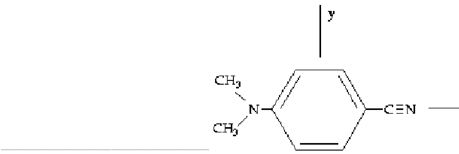
great accuracy is really required. The results for DMABN n C2v symmetry are compiled
in Table ![[*]](crossref.png) .
.
|
Fitting these values to a curve we obtain an optimal displacement of -1.0 au. We move the
molecule and reoptimize the cavity radius at the new position of the
molecule. The results are listed in Table .
|
There is no significant change. The cavity radius is then selected as 13.8 au and the position of the molecule with respect to the cavity is kept as in the last calculation. The calculation is carried out with the new values. The SCF or RASSCF outputs will contain the information about the contributions to the solvation energy. The CASSCF energy obtained will include the reaction field effects and an analysis of the contribution to the solvation energy for each value of the multipole expansion:
Reaction field specifications:
------------------------------
~
Dielectric Constant : .388E+02
Radius of Cavity(au): .138E+02
Truncation after : 4
~
Multipole analysis of the contributions to the dielectric solvation energy
~
--------------------------------------
l dE
--------------------------------------
0 .0000000
1 -.0013597
2 -.0001255
3 -.0000265
4 -.0000013
--------------------------------------
10.6.4 Solvation effects in ground states. PCM model in formaldehyde.
The reaction field parameters are added to the SEWARD program input through the keyword
RF-Input
To invoke the PCM model the keyword
PCM-model
is required. A possible input is
RF-input
PCM-model
solvent
acetone
AAre
0.2
End of rf-input
which requests a PCM calculation with acetone as solvent, with tesserae
of average area
 . Note that the default parameters are
solvent=water, average area
. Note that the default parameters are
solvent=water, average area
 ; see the SEWARD
manual section for further PCM keywords. By default the PCM adds
non-electrostatic terms (i. e. cavity formation energy, and dispersion
and repulsion solute-solvent interactions) to the computed free-energy
in solution.
; see the SEWARD
manual section for further PCM keywords. By default the PCM adds
non-electrostatic terms (i. e. cavity formation energy, and dispersion
and repulsion solute-solvent interactions) to the computed free-energy
in solution.
A complete input for a ground state CASPT2 calculation on formaldehyde
( ) in water is
&GATEWAY
Title
formaldehyde
Coord
4
H 0.000000 0.924258 -1.100293 Angstrom
H 0.000000 -0.924258 -1.100293 Angstrom
C 0.000000 0.000000 -0.519589 Angstrom
O 0.000000 0.000000 0.664765 Angstrom
Basis set
6-31G*
Group
X Y
RF-input
PCM-model
solvent
water
end of rf-input
End of input
&SEWARD
End of input
&SCF
Title
formaldehyde
Occupied
5 1 2 0
End of input
&RASSCF
Title
formaldehyde
nActEl
4 0 0
Inactive
4 0 2 0
Ras2
1 2 0 0
LumOrb
End of input
&CASPT2
Frozen
4 0 0 0
RFPErt
End of input
10.6.5 Solvation effects in excited states. PCM model and acrolein.
In the PCM picture, the solvent reaction field is
expressed in terms of a polarization charge density  spread
on the cavity surface, which, in the most recent version of the method,
depends on the electrostatic potential
spread
on the cavity surface, which, in the most recent version of the method,
depends on the electrostatic potential
 generated by the solute on the cavity according to
![$\displaystyle \left[ \frac{\epsilon+1}{\epsilon-1} \hat S
-\frac{1}{2\pi}\hat S \hat D^* \right]
\sigma(\bf s)$](img345.png)
![$\displaystyle \left[ - 1 + \frac{1}{2\pi} \hat D \right] V(\bf s)$](img346.png)
where
 is the solvent dielectric constant and
is the (electronic+nuclear) solute potential at point
is the solvent dielectric constant and
is the (electronic+nuclear) solute potential at point
 on the cavity surface.
The
on the cavity surface.
The  and
and  operators are related respectively to
the electrostatic potential
operators are related respectively to
the electrostatic potential
 and to the normal component of the
electric field
and to the normal component of the
electric field
 generated by the surface charge density .
It is noteworthy that in this PCM formulation the polarization charge
density is designed to take into account implicitly
the effects of the fraction of solute electronic density lying outside the
cavity.
generated by the surface charge density .
It is noteworthy that in this PCM formulation the polarization charge
density is designed to take into account implicitly
the effects of the fraction of solute electronic density lying outside the
cavity.
In the computational practice, the surface charge distribution
is expressed in terms of a set of point charges  placed
at the center of each surface tessera, so that operators are replaced by the
corresponding square matrices.
Once the solvation charges (q) have been determined,
they can be used to compute energies and properties in solution.
placed
at the center of each surface tessera, so that operators are replaced by the
corresponding square matrices.
Once the solvation charges (q) have been determined,
they can be used to compute energies and properties in solution.
The interaction energy between the solute and the solvation charges can be written
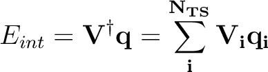 |
(10.6) |
 : since the charges
depend in turn on through the electrostatic potential, the solute
density and the charges must be adjusted until self consistency.
It can be shown[282] that for any SCF procedure including a
perturbation linearly depending on the electron density,
the quantity that is variationally minimized corresponds to a free energy
(i.e. Eint minus the work spent to polarize the dielectric and to create
the charges).
If
: since the charges
depend in turn on through the electrostatic potential, the solute
density and the charges must be adjusted until self consistency.
It can be shown[282] that for any SCF procedure including a
perturbation linearly depending on the electron density,
the quantity that is variationally minimized corresponds to a free energy
(i.e. Eint minus the work spent to polarize the dielectric and to create
the charges).
If
![$E^0=E[\rho^0] + V_{NN}$](img355.png) is the solute energy in vacuo, the free energy
minimized in solution is
is the solute energy in vacuo, the free energy
minimized in solution is
![\begin{displaymath}
{\cal G} = E[\rho] + V_{NN} + \frac{1}{2} E_{int}
\end{displaymath}](img356.png) |
(10.7) |
 is the
solute electronic density for the isolated molecule, and is the
density perturbed by the solvent.
is the
solute electronic density for the isolated molecule, and is the
density perturbed by the solvent.
The inclusion of non-equilibrium solvation effects, like those occurring during electronic excitations, is introduced in the model by splitting the solvation charge on each surface element into two components: qi,f is the charge due to electronic (fast) component of solvent polarization, in equilibrium with the solute electronic density upon excitations, and qi,s, the charge arising from the orientational (slow) part, which is delayed when the solute undergoes a sudden transformation.
The photophysics and photochemistry of
acrolein are mainly controlled by the relative position of the
 ,
,  and
and  states, which is,
in turn, very sensitive to the presence and the nature of the solvent.
We choose this molecule in order to show an example of how to
use the PCM model in a CASPT2 calculation of vertical excitation
energies.
states, which is,
in turn, very sensitive to the presence and the nature of the solvent.
We choose this molecule in order to show an example of how to
use the PCM model in a CASPT2 calculation of vertical excitation
energies.
The three states we want to compute are low-lying singlet
and triplet excited states of the s-trans isomer.
The  space (4 MOs /4 -electrons)
with the inclusion of the lone-pair MO (ny) is a suitable choice
for the active space in this calculation.
For the calculation in aqueous solution, we need first to compute the CASPT2
energy of the ground state in presence of the solvent water.
This is done by including in the SEWARD input for the corresponding gas-phase
calculation the section
space (4 MOs /4 -electrons)
with the inclusion of the lone-pair MO (ny) is a suitable choice
for the active space in this calculation.
For the calculation in aqueous solution, we need first to compute the CASPT2
energy of the ground state in presence of the solvent water.
This is done by including in the SEWARD input for the corresponding gas-phase
calculation the section
RF-input
PCM-model
solvent
water
DIELectric constant
78.39
CONDuctor version
AARE
0.4
End of rf-input
If not specified, the default solvent is chosen to be water.
Some options are available. The value of the dielectric constant
can be changed for calculations at temperatures other than 298 K.
For calculations in polar solvents like water, the use of the conductor
model (C-PCM) is recommended.
This is an approximation that employs conductor rather than dielectric
boundary conditions. It works very well for polar solvents
(i. e. dielectric constant greater than about 5), and is based
on a simpler and more robust implementation. It can be useful also in cases when
the dielectric model shows some convergence problems.
Another parameter that can be varied in presence of convergency problem
is the average area of the tesserae of which the surface of the cavity is composed.
However, a lower value for this parameter may give poorer results.
Specific keywords are in general needed for the other modules to work with PCM, except for the SCF. The keyword NONEquilibrium is necessary when computing excited states energies in RASSCF. For a state specific calculation of the ground state CASSCF energy, the solvent effects must be computed with an equilibrium solvation approach, so this keyword must be omitted. None the less, the keyword RFpert must be included in the CASPT2 input in order to add the reaction field effects to the one-electron hamiltonian as a constant perturbation.
&RASSCF &END
Title
Acrolein GS + PCM
Spin
1
Symmetry
1
nActEl
6 0 0
Frozen
4 0
Inactive
8 0
Ras2
1 4
LUMORB
THRS
1.0e-06 1.0e-04 1.0e-04
ITERation
100 100
End of input
&CASPT2 &END
Title
ground state + PCM
RFpert
End of Input
Information about the reaction field calculation employing a PCM-model appear first in the SCF output
Polarizable Continuum Model (PCM) activated
Solvent:water
Version: Conductor
Average area for surface element on the cavity boundary: 0.4000 Angstrom2
Minimum radius for added spheres: 0.2000 Angstrom
Polarized Continuum Model Cavity
================================
Nord Group Hybr Charge Alpha Radius Bonded to
1 O sp2 0.00 1.20 1.590 C [d]
2 CH sp2 0.00 1.20 1.815 O [d] C [s]
3 CH sp2 0.00 1.20 1.815 C [s] C [d]
4 CH2 sp2 0.00 1.20 2.040 C [d]
------------------------------------------------------------------------------
The following input is used for the CASPT2 calculation of the
 state.
Provided that the same $WorkDir has been using, which contains all the files of of the
calculation done for the ground state, the excited state calculation is done
by using inputs for the RASSCF
and the CASPT2 calculations:
state.
Provided that the same $WorkDir has been using, which contains all the files of of the
calculation done for the ground state, the excited state calculation is done
by using inputs for the RASSCF
and the CASPT2 calculations:
&RASSCF &END
Title
Acrolein n->pi* triplet state + PCM
Spin
3
Symmetry
2
nActEl
6 0 0
Frozen
4 0
Inactive
8 0
Ras2
1 4
NONEquilibrium
LUMORB
ITERation
100 100
End of input
&CASPT2 &END
Title
triplet state
RFpert
End of Input
Note the RASSF keyword NONEQ, requesting that the slow part of the reaction field be frozen as in the ground state, while the fast part is equilibrated to the new electronic distribution. In this case the fast dielectric constant is the square of the refraction index, whose value is tabulated for all the allowed solvents (anyway, it can be modified by the user through the keyword ``DIELectric'' in SEWARD).
The RASSCF output include the line:
Calculation type: non-equilibrium (slow component from JobOld)
Reaction field from state: 1
This piece of information means that the program computes the solvent
effects on the energy of the
by using a non-equilibrium approach.
The slow component of the solvent response is kept frozen in terms of the charges
that have been computed for the previous equilibrium calculation of
the ground state. The remaining part of the solvent response,
due to the fast charges, is instead computed self-consistently for the
state of interest (which is state 1 of the specified spatial and spin symmetry in this case).
The vertical excitations to the lowest valence states
in aqueous solution for s-trans acrolein are
listed in the Table and compared
with experimental data.
As expected by qualitative reasoning, the vertical excitation energy to the
 state exhibits a blue shift in water.
The value of the vertical transition energy computed with the inclusion of the
PCM reaction field is computed to be 3.96 eV at the CASPT2 level of theory.
The solvatochromic shift is thus of +0.33 eV.
Experimental data are available for the
excitation energy to the
state. The band shift in
going from isooctane to water is reported to be +0.24 eV which is in fair
agreement with the PCM result.
state exhibits a blue shift in water.
The value of the vertical transition energy computed with the inclusion of the
PCM reaction field is computed to be 3.96 eV at the CASPT2 level of theory.
The solvatochromic shift is thus of +0.33 eV.
Experimental data are available for the
excitation energy to the
state. The band shift in
going from isooctane to water is reported to be +0.24 eV which is in fair
agreement with the PCM result.
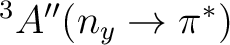
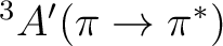
No experimental data are available for the excitation energies to the triplet
states of acrolein in aqueous solution. However it is of interest to see how
the ordering of these two states depends on solvent effects.
The opposing solvatochromic shifts produced by the solvent on these two electronic transitions
place the two triplet states closer in energy.
This result might suggest that a dynamical interconversion between
the  and
and  may occur more favorable in solution.
| State | Gas-phase | Water | Expt.a |
 |
3.63 | 3.96 (+0.33) | 3.94 (+0.24)b |
T1
 |
3.39 | 3.45 (+0.06) | |
T2
 |
3.81 | 3.71 (-0.10) | |
| aRef.[285] | |||
| bSolvatochromic shifts derived by comparison of the absorption wave lengths in water and isooctane | |||
Next: 10.7 Computing relativistic effects in Up: 10. Examples Previous: 10.5 Excited states.